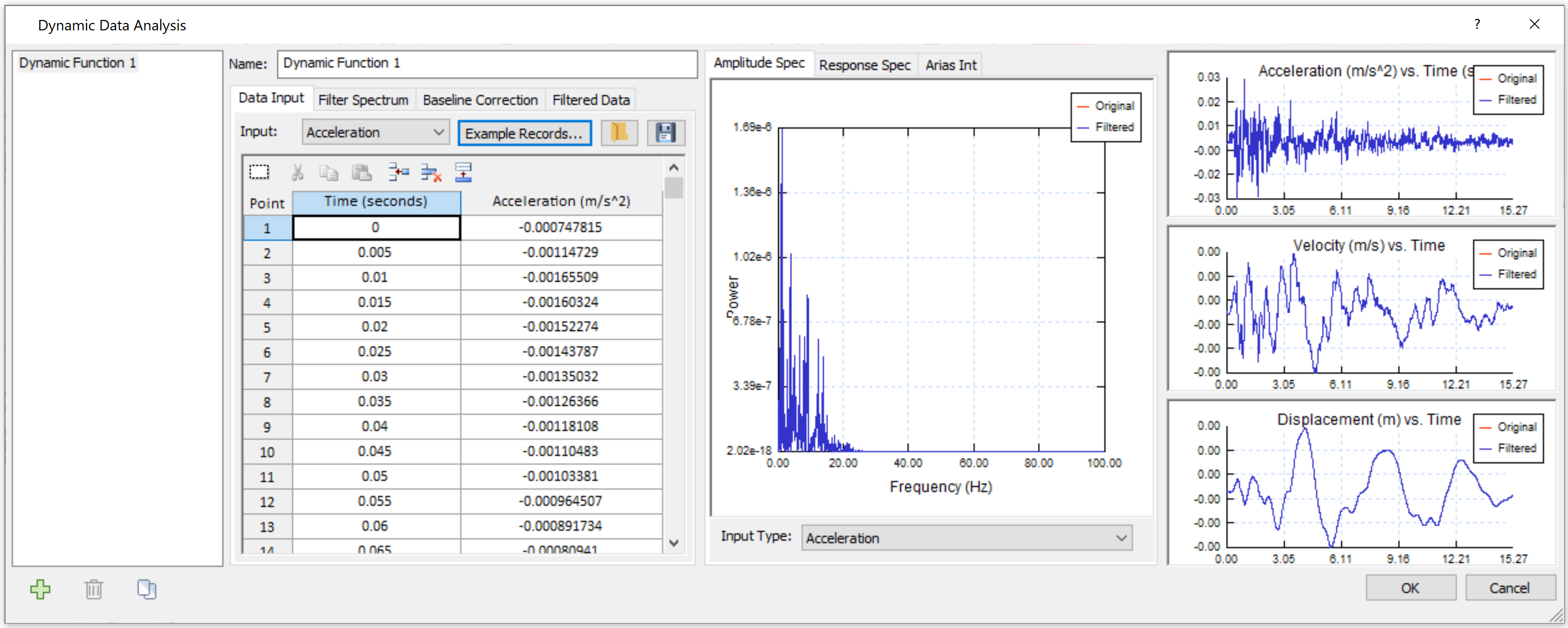
Dynamic Data Analysis

The Dynamic Data Analysis option in RS2 allows you to perform analysis on input dynamic data. The analysis presents data information, provides means of modifications to increase data accuracy and stability, and outputs a set of new data. Four sections are provided for Dynamic Data Analysis: Data Input, Filter Spectrum, Baseline Correction, and Filtered Data, as described in detail below.

To use the option:

1. Ensure Dynamic Analysis is enabled in Project Setting menu.
2. Select Dynamic > Dynamic Data Analysis.
3. In the Dynamic Data Analysis dialog, the dynamic functions will be listed in the left panel of the dialog. You can add a dynamic function with the Add button , delete with the Delete button , and copy the function with the Copy button . You can edit the dynamic function name.
4. Along the analysis, the right panel of the dialog provides several plots to monitor the state and change of data graphically: Amplitude Spectrum, Response Spectrum, Arias Intensity, and time histories for displacement, velocity, and acceleration.
5. Follow the sequence of Data Input, Filter Spectrum, and Baseline Correction tabs to perform analysis. The output data after modifications will display under the Filtered Data tab.
6. Click OK in the dialog when complete. The output data can then be applied using the Define Dynamic Loads option.

Another way to access the Dynamic Data Analysis feature is within the Define Dynamic Loads dialog:

1. Ensure Dynamic Analysis is enabled in Project Setting menu.
2. Select Dynamic > Define Dynamic Loads.
3. In the Define Dynamic Loads dialog, if the Type is Displacement, Velocity, or Acceleration, then when you click the Define button , the Dynamic Data Analysis feature will be available to perform analysis on input data, as shown in the picture below.



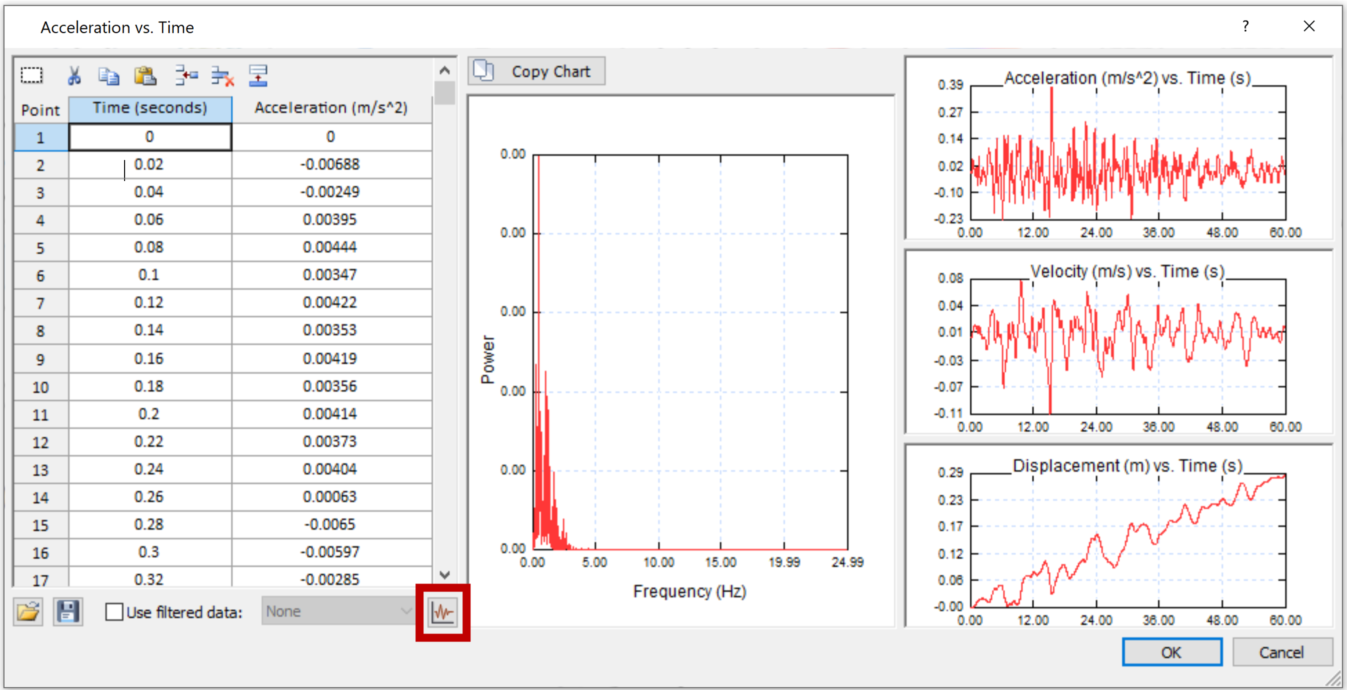
4. Click on the Dynamic Data Analysis button to modify the data.

Data Input

The Data Input tab allows you to input raw data.

1. Select the Input data type using the dropdown list. The supported dynamic data types include displacement, velocity, and acceleration.
2. There are several ways to input raw data:

   1. Use the data grid.

      You can use the tools above the grid section to select all , cut , copy , paste , insert row , delete row , and append row . If you have data copied, and want to paste to the grid. Click on the select all button , and click paste or ctrl+v. Data will be pasted to the grid.

   2. Use the example earthquake records provided by RS2.

      Select the Example Records button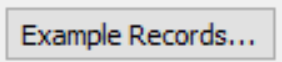 . A list of example earthquake records with their properties will be displayed in the dialog. Make you selection and click OK in the dialog to apply. The data will be automatically loaded to the grid.

   3. Load function from file

      To load dynamic data from a file, select the Load button . Select a file and click Open. A dialog will pop up for unit conversion as shown below.

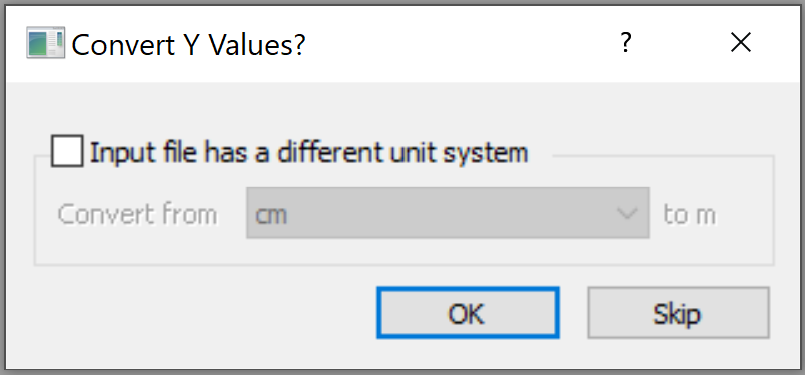
      This dialog is to align the unit system of the Y value to the model. If the file data has a different unit system from the model, select the checkbox for Input file has a different unit system. Use the dropdown list to choose the unit system of the file data to perform conversion, and select OK to apply.

      Select Skip in the dialog if the Y value unit in the data file is the same as the model.

3. You can use the Save button to save input data to file.

Filter Spectrum

The Filter Spectrum tab can be used after data input. It allows you to select the natural frequency range based on power distribution over frequency components. The chosen range should include the majority of the data, as well as the important data points. The amplitude spectrum (Power vs. Frequency (Hz)) data is generated in the data grid and the graph.

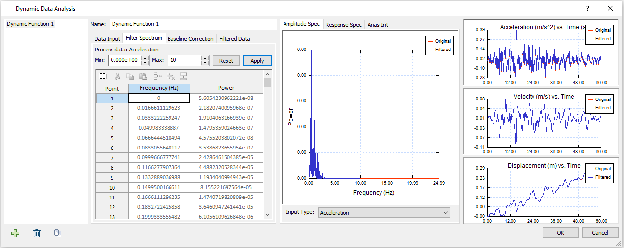
1. Under the Amplitude Spectrum tab for graphs, select the Input Type (velocity or acceleration) using the dropdown list. A Fast Fourier Transform (FFT) will then be applied to convert the data to a power spectrum, as shown in the data grid and the amplitude spectrum plot.
2. Users can set a range by stating the minimum and maximum frequency in the dialog. Click Apply, the new range will be updated to both the data and graphs. Click Reset to go back to the original range.
3. After setting the range, select Apply, and proceed to the Baseline Correction tab.

Baseline Correction

The Baseline Correction option allow you to correct data drift. Tow methods are available: Cutoff and Sinusoid. Cutoff is available to correct only velocity drift, sinusoid is available to correct both velocity and displacement drift.

1. Select the data type that you would like to correct the drift from Process Data.
2. Select the Method as either Cutoff or Sinusoid.
• Cutoff Method
1. For Cutoff method, the Applicable Cut Off Range will be displayed.
   
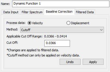
2. A reference Cutoff value will be generated for the user that outputs the optimal baseline correction. User can edit the Cutoff value.
3. Click Apply to apply the Cutoff value. The change will be applied to the data and shown on plots.
4. The Undo button allows you to take a step back.
• Sinusoid Method
1. For Sinusoid method, a Residual Value will be generated, as well as a reference Manual Correction value. User can edit the Manual Correction value.
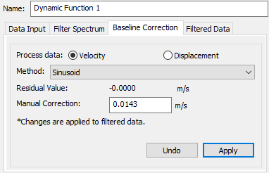
2. Click Apply to apply the Manual Correction value.
3. The correction will be applied to the data and shown on plots. The Residual Value will also be updated. A residual value of 0 means the baseline has been corrected to zero.
4. The Undo button allows you to take a step back.
3. When finishing baseline correction, proceed to the Filtered Data tab.

Filtered Data

The Filtered Data tab presents the output data after the modifications from Filtered Spectrum and Baseline Correction. Users can select the Output Data type as Acceleration, Velocity, or Displacement, using the dropdown list.

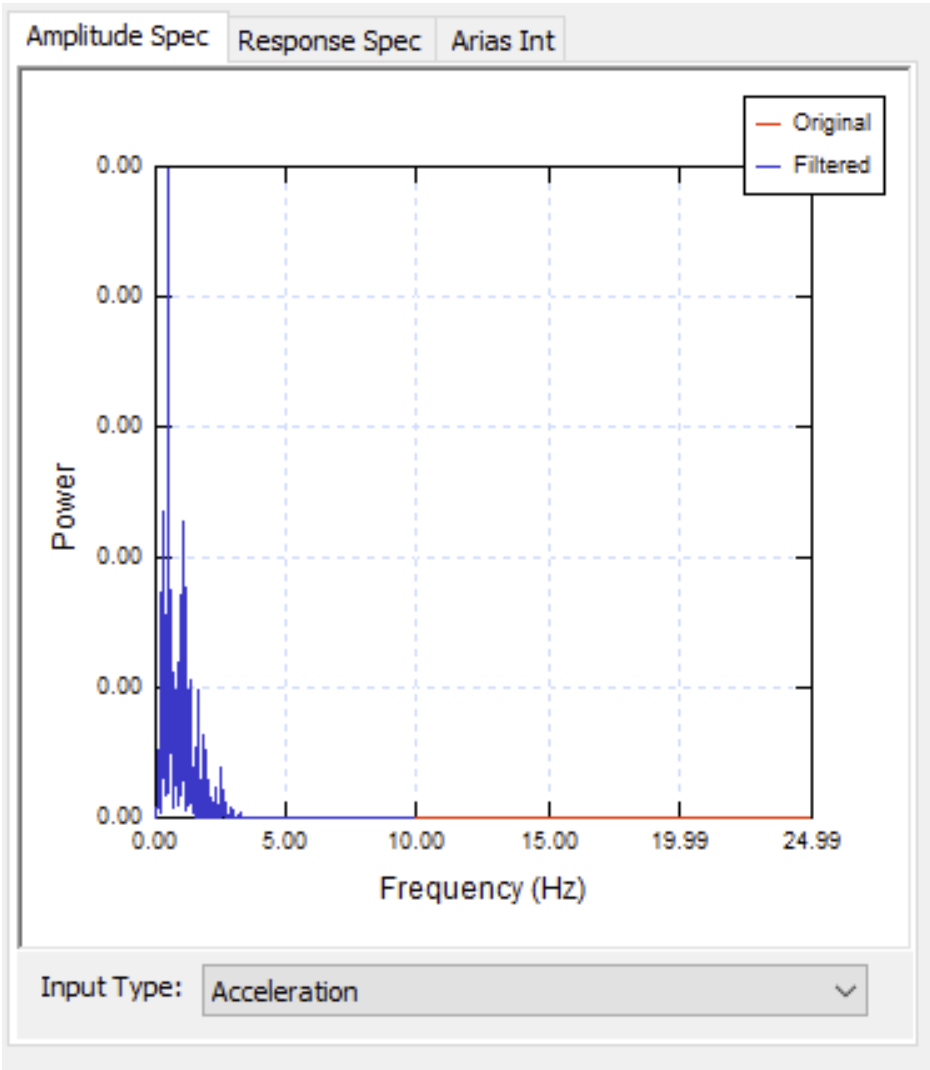
Plots

Once the dynamic function time histories are entered under the Input Data tab, several graphs will be automatically generated and displayed in the dialog: Amplitude Spectrum, Response Spectrum, Arias Intensity, Time-acceleration history, Time-Velocity history, and Time-displacement history.

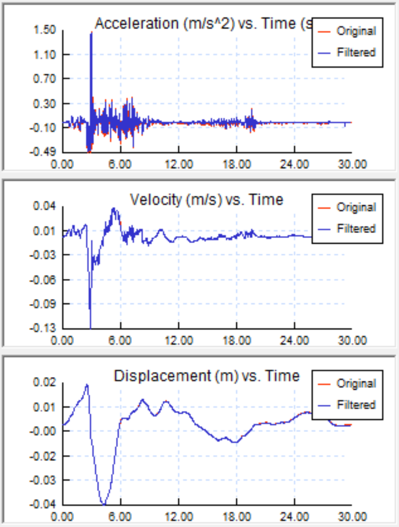
The change of the data can be monitored and compared with raw data in these graphs. The updated data will be plotted as in color blue, and the original data will be plotted in color red.

Amplitude Spectrum

The amplitude spectrum (power spectrum) shows the power distribution over frequency processed from the input data type of Acceleration or Velocity based on user’s choice.

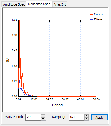
Response Spectrum

The Response Spectrum estimates the structural response to an input motion during dynamic events. It is a plot of Spectral Acceleration vs. Period. Users can modify the maximum period and the damping ratio to observer the response. Click Apply to observe and compare the change.

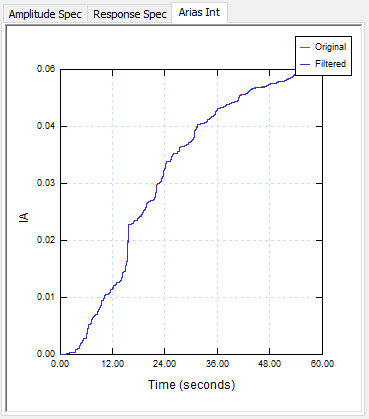
Arias Intensity

The Arias Intensity vs. Time graph is generated for the user to observe the Arias intensity change over time.

Time History Graphs

The Acceleration-time history, Velocity-time history, and Displacement-time history are also plotted as shown below.

For more information about Dynamic Data Analysis:

• See RS2 Dynamic Analysis Theory Manual for theories and equations
• See RS2 Dynamic Data Analysis Tutorial for an example with detailed steps.