Interpolation Method

There are many different methods which can be used to interpolate values from a grid of data specified at X , Y,and Z locations. Interpolation implies that the value of a variable can be determined at any required location, based on the defined values at specified locations.

In RS3, Interpolation Methods are used for:

• Interpolating values of pore pressure if the Static Water Mode is set to Grid. See the Groundwater Method topic for details. The Interpolation Method is used to obtain the value of pore pressure at each node of the finite element mesh, based on the water pressure data at the grid points. The pore pressure at the mesh nodes can then be used directly in the finite element analysis.
• Interpolating values of strength function parameters (cohesion, friction angle, modulus) when using the Discrete Strength Function option in the Define Material Properties dialog. See the Discrete Strength Function topic for details.

The following Interpolation Methods are available in RS3.

Inverse Distance

The Inverse Distance Interpolation method weights every grid point according to its distance from the sample point. This scheme is also known as the Shepard method (Shepard, 1968) and can be written in the form:

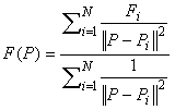
where P is the location of the sample point, F(P) is the interpolated value at the sample point, Pi the location of the grid points, Fi are the grid point values, and ||P-Pi||2 represents the distance from P to Pi. The main deficiencies of this method are: 1) the local extrema are typically located at the grid points and this results in poor shape properties, and 2) undue influence of grid points which are far away from the sample point.

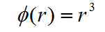
Thin Plate Spline

The Thin-Plate Spline method utilizes the concept of an infinite thin elastic plate under tension, to determine a spline surface (a smooth 3-dimensional surface which fits through all of the grid points). The spline surface is used to determine the sample value at any location (Franke, 1985).

Chugh’s Method

The Chugh interpolation method is based on finding the nearest grid point in each of the four quadrants with origin centered at the point where the interpolation is required. A plane is then fit through each combination of three quadrant grid points, and an interpolation is performed for each plane. This results in four interpolations, which are then averaged to obtain the final interpolated value at the desired point (Chugh, 1981).

Local Thin Plate Spline

The Local Thin Plate Spline method is an extension of the Thin Plate Spline interpolation technique, and is recommended for use with a large number of grid points (>200). The only difference between the methods is that instead of using all the grid points for the interpolation, the Local version takes a maximum of 10 closest points to the sample point and fits a spline surface through them. The local spline surface is then used to determine the sample value.

Linear By Elevation

The Linear by Elevation method only utilizes the elevation (y-coordinate) of each grid point. The method determines the closest grid point (elevation) above the sample point and the closest grid point (elevation) below the sample point, and linearly interpolates the sample value based on these two data points. Interpolation is done in the vertical direction only. This method is meant for horizontally bedded soils where data varies by depth only. It is very useful for cases where a complicated pore pressure profile exists in only the vertical direction. The x-coordinate of the grid points is not used in the interpolation process. However, it is used to display the data on your model.

Gaussian

Gaussian or Normal distribution is a commonly used radial basis function (Fornberg & Piret, 2008) that follows the form:

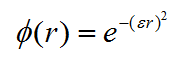
where:

is the influence of a data point to the interpolated point based on the distance between them denoted as r.

is similar to other radial basis functions such as thin-plate spline, the interpolated point is obtained by summing the weighted value are determined by the magnitude of the data point. In surface reconstruction, the magnitude of the data point is the elevation at the XY coordinate. In pore pressure interpolation, the weight would be pore pressure at the XYZ coordinate of the data point.

Multi Quadratic

Multi Quadratic radial basis function (Fornberg & Piret, 2008) used in Slide3 follows the form:

is the influence of a data point to the interpolated point based on the distance between them denoted as r.

is a shape parameter and is taken as the average distance between all data points. Similar to other radial basis functions such as thin-plate spline, the interpolated point is obtained by summing the weighted.

The weights for each value are determined by the magnitude of the data point. In surface reconstruction, the magnitude of the data point is the elevation at the XY coordinate. In pore pressure interpolation, the weight would be pore pressure at the XYZ coordinate of the data point.

Polyharmonic Spline

Polyharmonic spline radial basis function (Fornberg & Piret, 2008) used in Slide3 follows the form:

is the influence of a data point to the interpolated point based on the distance between them denoted as r. Thin-Plate Spline is a special case of the polyharmonic spline functions. Similar to other radial basis functions such as thin-plate spline, the interpolated point is obtained by summing the weighted values of all data points. The weights for each value are determined by the magnitude of the data point. In surface reconstruction, the magnitude of the data point is the elevation at the XY coordinate. In pore pressure interpolation, the weight would be pore pressure at the XYZ coordinate of the data point.

Compactly Supported

Compactly supported methods perform interpolation for a point in space using the closest data points within a specified radius. All data points outside of the specified radius have no influence on the interpolation for that specific point (Wendland, 1995). The compactly-supported radial basis function implemented in Slide3 to calculate the influence of a data point to the interpolation follows the form:

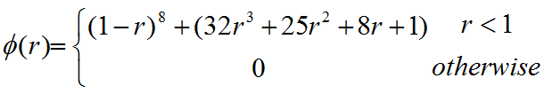
Where:

is the influence of a data point to the interpolated point based on the distance between them denoted as r. Similar to other radial basis functions such as thin-plate spline, the interpolated point is obtained by summing the weighted values of all data points. The weights for each value are determined by the magnitude of the data point. In surface reconstruction, the magnitude of the data point is the elevation at each XY coordinate.

For Porewater Pressure Grid:

Kriging

Kriging is a best linear unbiased estimator (BLUE), or a weighted average that minimizes the prediction error associated with the estimate. Ordinary Kriging is used in RS3, meaning that the mean is assumed to be constant but unknown (Baily and Gatrell, 1995). The weighted average equation is expressed as follows:

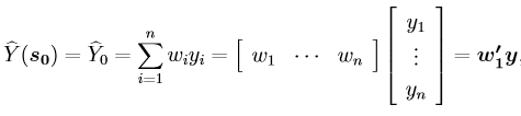
Where y is the vector of sampled values, and w’ is the vector of weights applied to the sampled values. The weights are based on the covariances between the sampled points, and the covariances between the sampled points and the point to be predicted. Slide uses an exponential semivariogram for estimating the covariances. For compatibility with a large number of data points, the kriging method takes a maximum of 50 closest points to the point to be predicted.