Trace Map Analysis

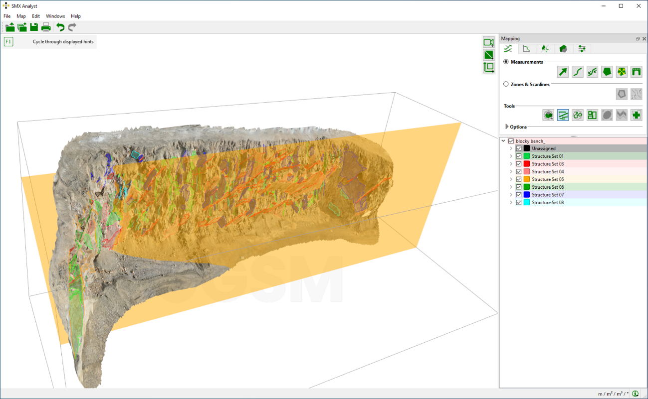
Trace Map Analysis in the Analyst shows data on trace spacing. This Structure Tool is controlled via the Trace Map Analysis dialog. The input data is defined by the entire Map or if defined Analysis Zones and Exclusions Zones. Considered Annotation Elements for analysis are Traces, Areas and Bridges. Results are displayed in a distribution plot (histogram).

Upon calling the Trace Map Analysis dialog, the Projection Plane of the Structure Set / Analysis Zone is displayed in the 3D viewer together with the bounding box enclosing the selected measurements. Projected Traces appear as non-parallel straight lines in the colour of the Structure Set.  Scanlines are outlined as dotted lines whereas the intersection points are indicated by a circle.

Standard operating procedure

1. Click on the “Trace Map Analysis” icon in the toolbar of the Structure tab of the Mapping pane or chose “Window | Trace Map Analysis” in the menu bar.
2. The Trace Map Analysis dialog appears revealing the analyzed data

The below figure shows a projected trace map of an entire Map. It is possible to switch between the Structure Sets by using the pull down menu. If Analysis Zones are defined it is possible to switch between individual zones by using the pull down menu

Spacing calculations consider Traces and Areas which are projected with their orientation onto a reference plane, i.e. Projection Plane, parallel to the mean orientation vector of the Structure Set. If a Trace has no orientation, the mean orientation of the Structure Set is used for the projection. The direction of the scanlines is parallel to the mean orientation of the Structure Set. The calculation of the Trace and Bridge lengths is based on the length along the surface. 

Single Traces can be selected in the Trace Map Analysis dialog by clicking with the left mouse button on the item. It is then highlighted in the projection, the Structure List and in the 3D viewer. Using the “Seek to” function from the context menu of the annotation, the item found on the 3D model. Multiple selection is performed by holding “Ctrl” and clicking the left mouse button on the desired items. The middle mouse button is used to pan plot. The same can be done by pressing “Ctrl” or “Shift” and using the left mouse button. Zooming is performed by using the wheel if the computer mouse.

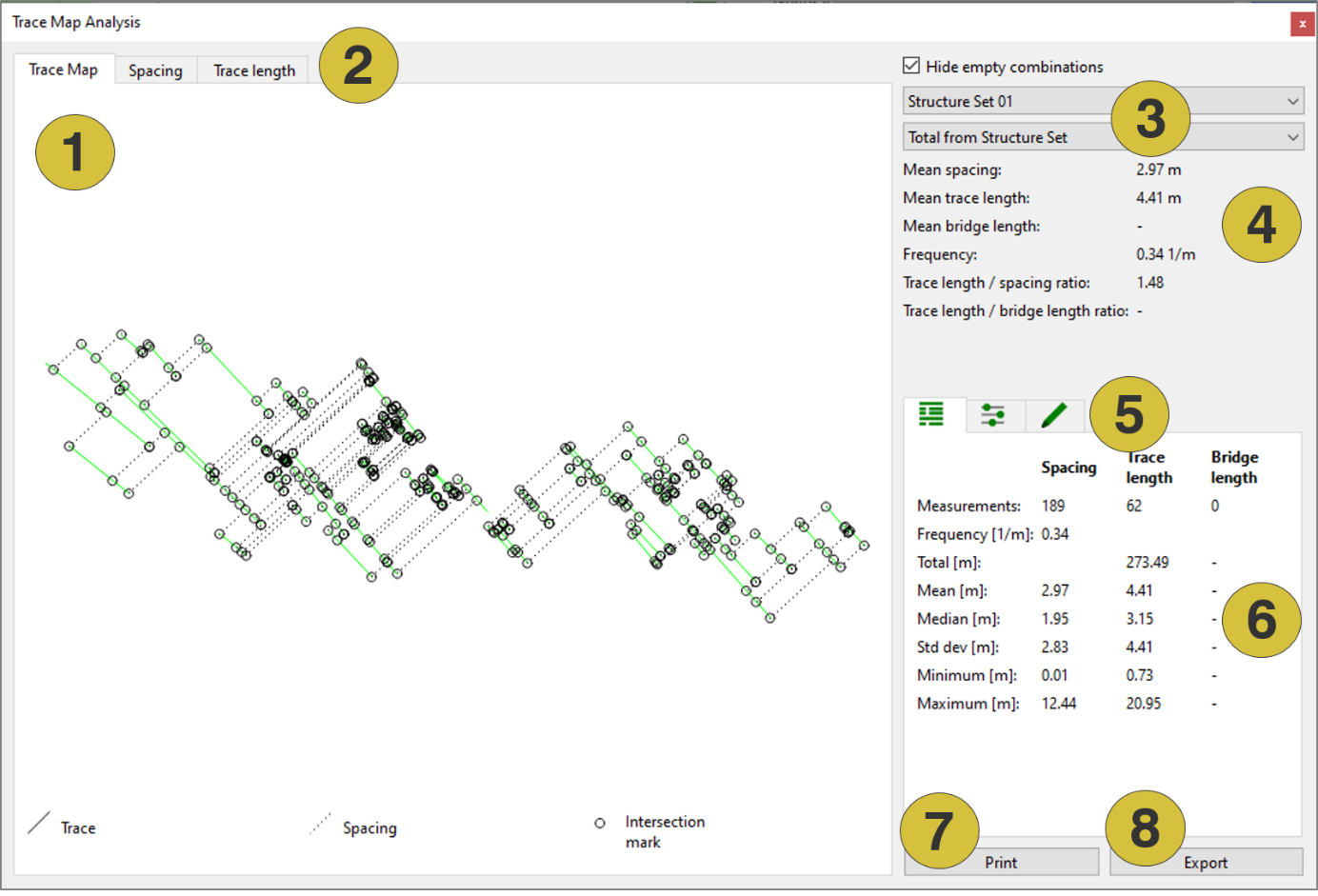
1. Projected trace map 
2. Distributions plots (available for Spacing, Trace Length and Bridge Length)
3. Pull down menu for switching between Structure Sets and Analysis Zones
4. Spacing and trace length statistics
5. Configuration tabs – Plot configuration and histogram configuration 
6. Parameters of spacing and trace length statistics
7. Print trace map and statistics
8. Export spacing and trace length data

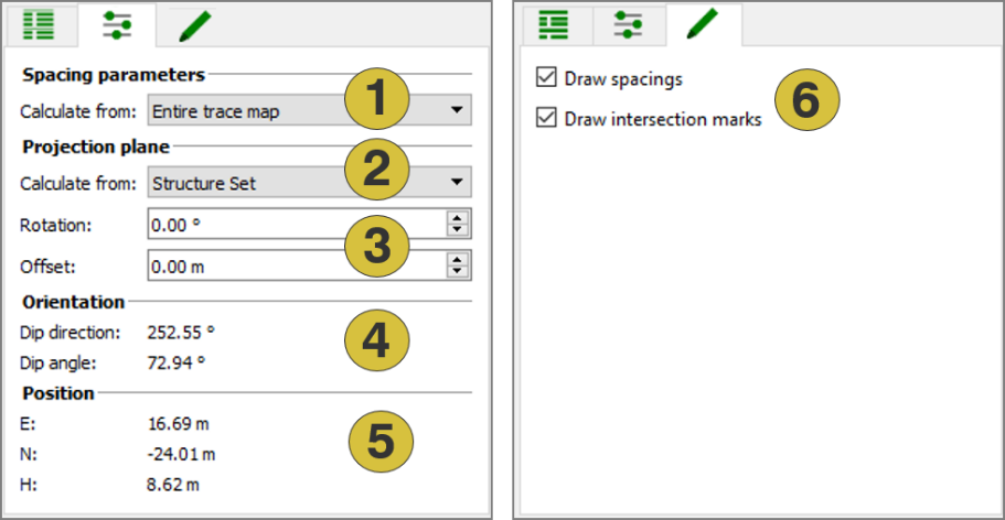
1. Configuration of spacing calculations
2. Configuration of calculating the Projection Plane
3. Rotation and Offset of the Projection Plane
4. Dip direction and angle of the Projection Plane
5. Position of the Projection Plane
6. Plot 

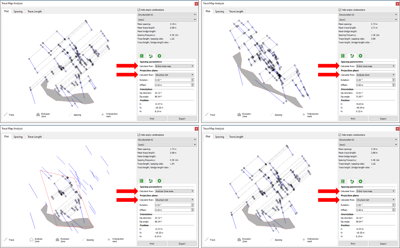
The statistics can be printed by clicking “Print” button and/or is written to a file in “.csv” format by clicking “Export”  button in the Trace Map Analysis dialog. The “.csv” files can be imported by any spread sheets application like MS Excel. The structure of the “.csv” export data file is the following: 

• Header row: Structure Set Information
  Structure Set, Selection, Dip direction (projection plane)[°], Dip angle of (projection plane)[°], E (projection plane)[m], N (projection plane)[m], H (projection plane)[m]
• Header row: Statistics
  Number of measurements, Frequency [1/m],Spacing measurements [m],Mean[m], Median [m], Standard deviation [m], Minimum [m], Maximum [m], Measurements [m]

Distribution plot

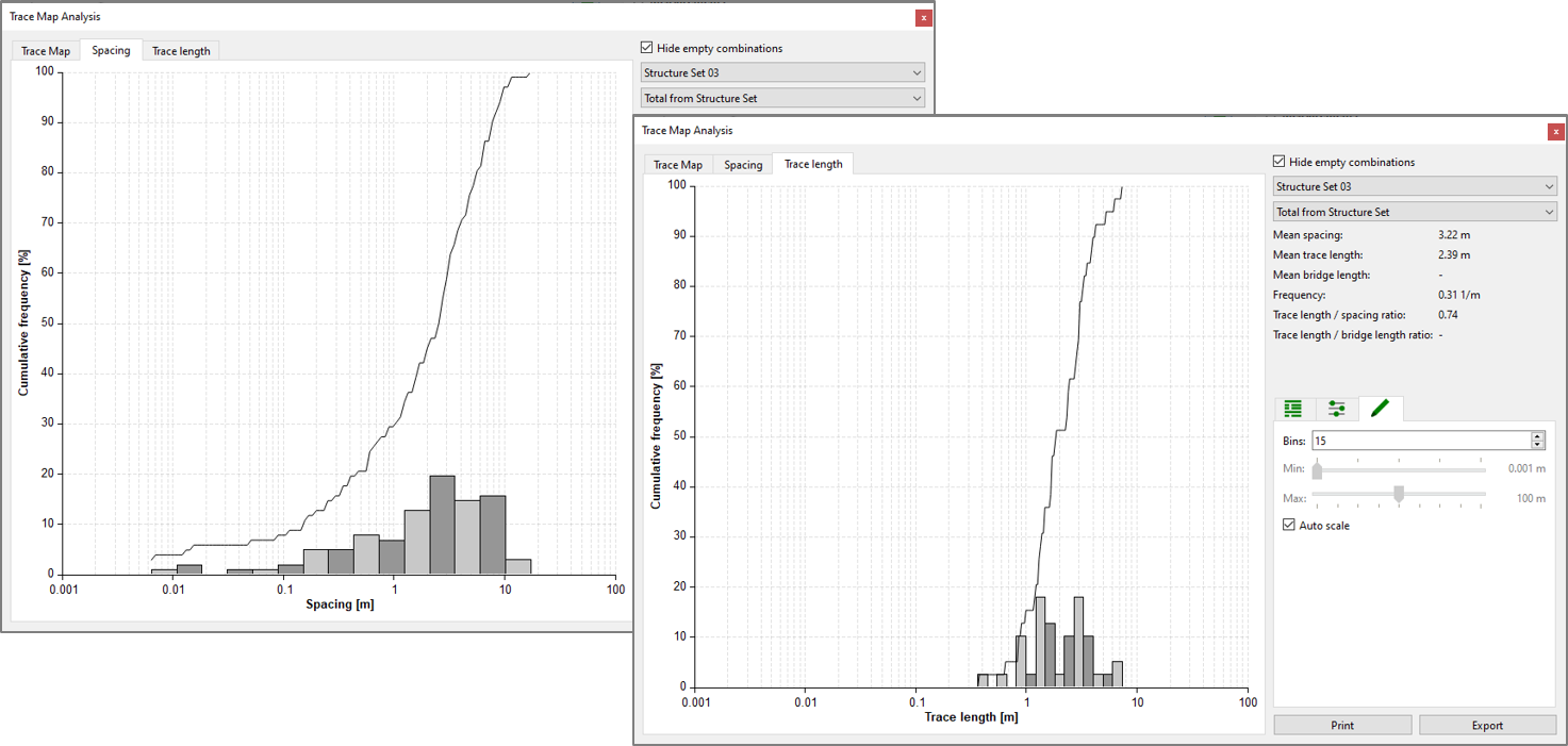
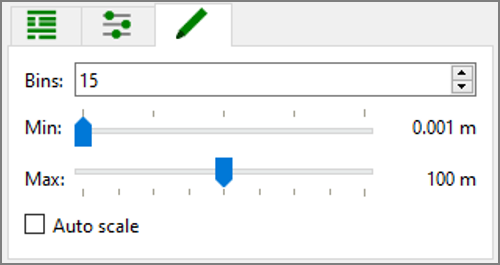
The distribution of Spacing, Trace Length and Bridge Length is visualized by plotting the cumulative relative length according to the total length. The individual plots are found in the corresponding tabs. The representation of the distribution is shown in a histogram that is configurable by the user in the Histogram Configuration tab. The number of bins as well as the scaling can be adapted.

Context menu of the plot

• Show Grid - Shows/hides the grid
• Show Tick Values - Shows/hides tick values
• Show Axis Label - Shows/hides the axis labels
• Save - Saves the current image as “.jpg” file