Stereonet Analysis

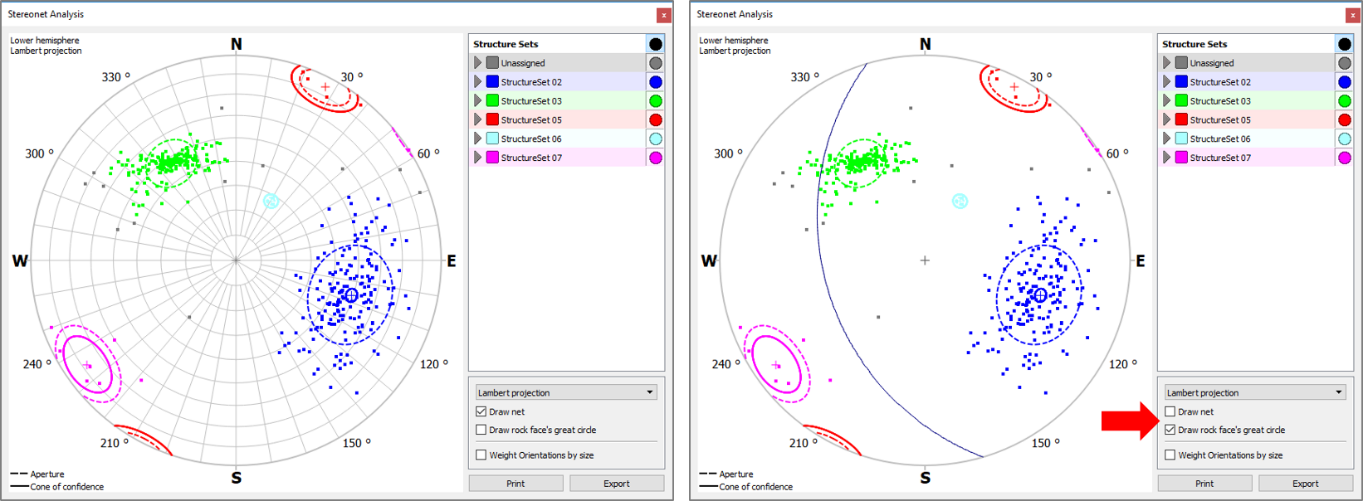
The Stereonet Analysis in the Analyst shows the poles of measured Orientations discriminated for each Structure Set in a hemispherical plot. In addition to the graphical representation, orientation statistics for each Structure Set is given. Orientation measurements and statistics are displayed in the projection as poles and cones, respectively. Poles are drawn as dots in which the selected Orientation is highlighted. The cone of confidence is represented as a solid small circle. The spherical aperture is represented as a dashed small circle. The circle are displayed in the plot in the colour of the corresponding Structure Set. The Hemispherical Plot shows only Orientations which are enabled in the Structure List.

Standard operating procedure

1. Click on the “Stereonet Analysis” icon in the toolbar of the Structure tab of the Mapping pane or chose “Window | Stereonet Analysis” in the menu bar
2. The Stereonet Analysis dialog appears showing the projection and the corresponding orientation statistic of each Structure Set

Two types of projections are available: 

• Lambert Projection for equal area projection
• Stereographic Projection for equal angle projection

The projection type is selectable in the pull down menu in the Stereonet Analysis dialog. By definition, the projections are displayed is the lower hemisphere (upper focal point). 

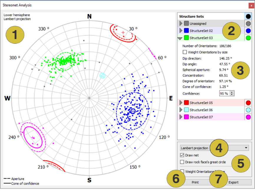
1. Projection of the lower hemisphere                      
2. Individual Structure Sets
3. Information and statistics to individual Structure Sets
4. Type of projection
5. Options
6. Print projection and statistics
7. Export projection and statistics

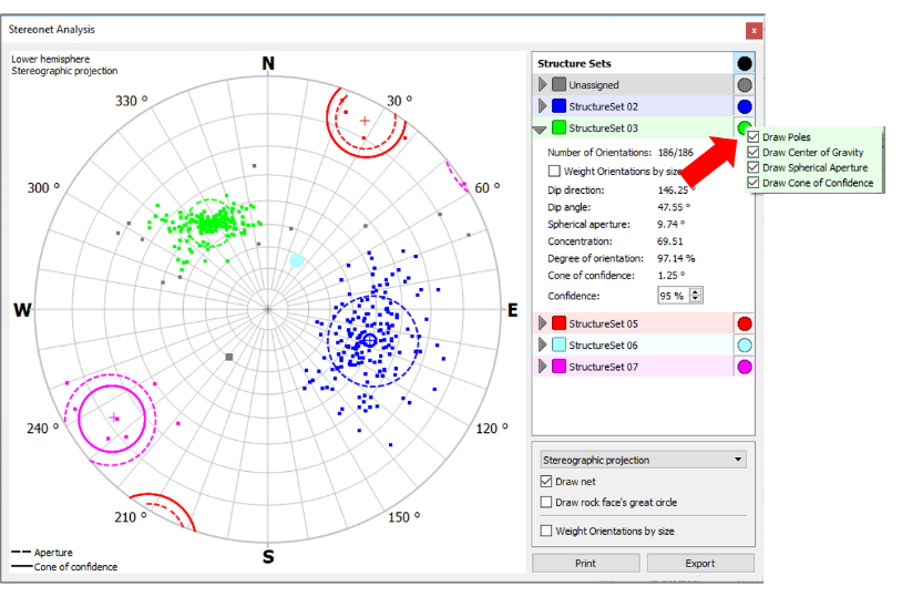
The Structure Set header allows configuring the display of the projection. The poles and statistics of an entire Structure Set can be turned off and off by clicking the radio button on right hand side of the header. The poles, the center of gravity, the circles for spherical aperture (dashed line) and cone of confidence (solid line) can be individually enabled and disabled by clicking with the right mouse button on radio button and ticking the corresponding checkboxes.

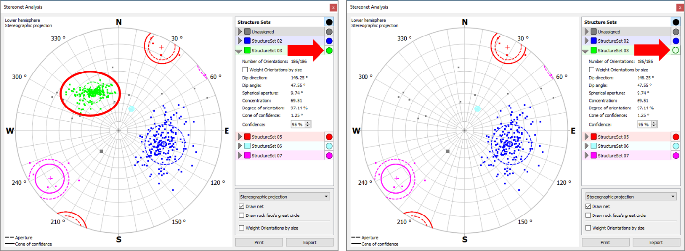
The Structure Set header is followed by the Orientation Statistics. Following information and statistic is provided:

• Number of Orientations: Active number / Total number
• Weight Orientations by Size: The mean orientation vector of a Structure Set is the vector sum of all Orientation measurements contained in the Structure Set and divided by the number of measurements. This calculation assumes equal weights for each measurement and neglects the large joints may have more impact on the mean set orientation than small joints. Analyst allows to enable weights for each measurements. The weights are related to the maximum diameter of the structure. In consequence, large structures have more impact on the mean set orientation than small structures. The mean orientation vector of a Structure Set is then the sum of all weighted Orientation measurements contained in the Structure Set. “Weight Orientations by size” is enabled by ticking the corresponding checkbox. 

• Dip direction: mean value for a Structure Set
• Dip angle: mean value for a Structure Set
• Spherical aperture: spread of the Orientations around the mean value. It is comparable with the standard deviation for linear statistics
• Concentration: compares the Orientation sample size with the length of the mean orientation vector. The longer the vector for the same samples size the higher is the concentration. It describes the concentration of Orientations around a mean orientation value. Concentration = 0 describes a uniform distribution. Concentration equals Fisher’s constant.
• Degree of orientation: normalised measure for the alignment of orientations. 0% means uniform distribution of Orientations, 100% means parallel alignment.
• Cone of confidence: defines a confidence region (small circle) around the calculated mean orientation which delimits the deviation of the true mean orientation for a certain level of confidence. If the confidence level is high, the cone of confidence is also large.
• Confidence: defines a level of certainty or probability, respectively, for the interpretation of results from statistical calculations. Higher levels of confidence include a wider spread compared to smaller levels. The confidence level can be edited in the dialog.

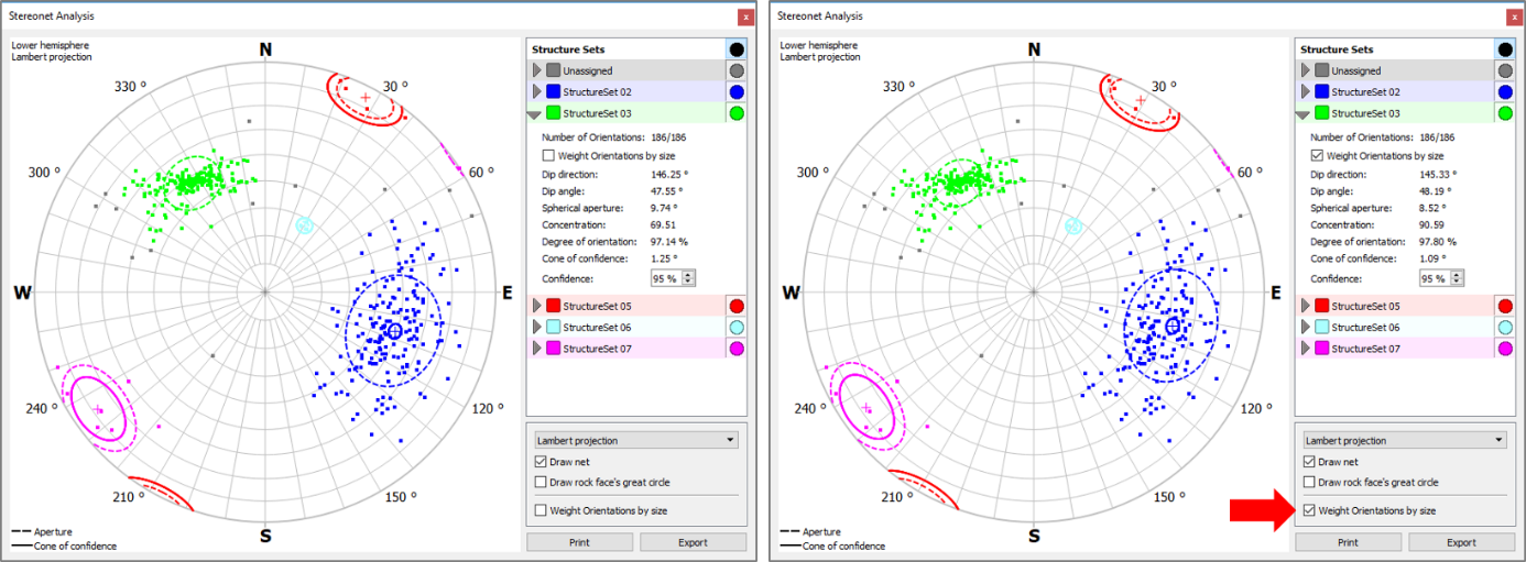
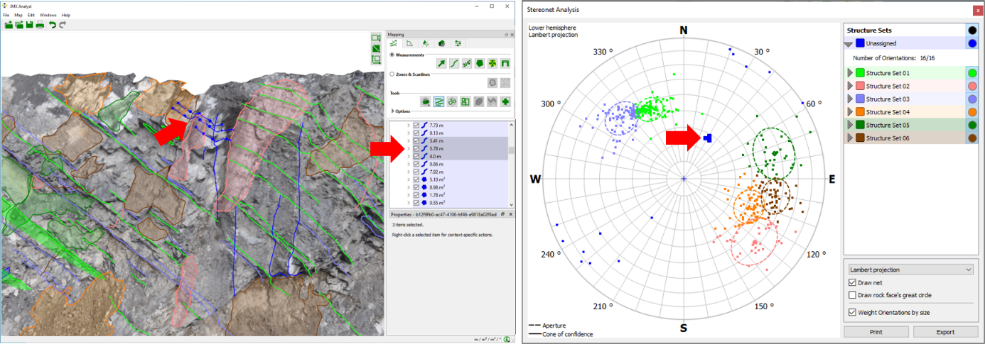
Single orientation poles can be selected in the hemispherical plot by clicking with the left mouse button on the pole. It is then highlighted in the plot, the Structure List and the 3D viewer. Using the “Seek to” function from the context menu of the annotation, the Orientation is found on the 3D model. Multiple selection of poles is performed by holding “Ctrl” and clicking the left mouse button on the desired items.

The hemispherical plot is saved as image (“.png” file) by clicking with the right mouse button somewhere in the viewer. A click on “Save as Image” opens a dialog to title the plot and to select the directory so save on the computer. Statistics can be printed using the “Print” button or exported to a file in “.csv” format using the “Export” button. The “.csv” files can be imported by any spread sheet application like MS Excel. The file starts with a header row, then following a row containing the name of the Structure Set, a row with the Structure Set statistics, and then several rows with the individual Orientation measurements. Any subsequent Structure Sets are separated by a blank row. The decimal point is the comma while the separator is the semicolon (in the English version of the software). The structure of the “.csv” export data file is the following: 

• Header row (one per file):
  dip direction, dip angle, spherical aperture, concentration parameter, percentual degree of orientation, cone of confidence, confidence, number of orientations
• Structure Set row (one per Structure Set):
  Structure Set name
• Statistic row (one per Structure Set):
  2 numerical values: dip direction, dip angle