Conditional Random Fields
Condition Random Field is a sub-option of Probabilistic Analysis in Slide2. A Conditional Random Field (CRF) is a spatial field that has been adjusted based on known observed data, typically in the form of borehole data such as SPT or CPT. Conceptually, the introduction of known measured data allows the generated spatial field to approach a truer representation of the real physical field, enhancing accuracy in analyses.
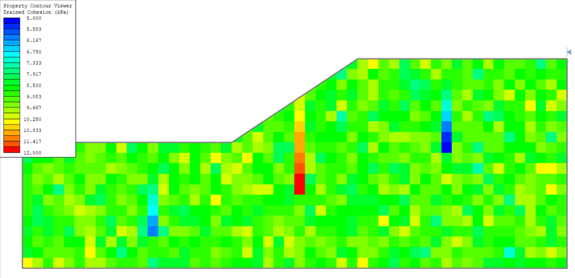
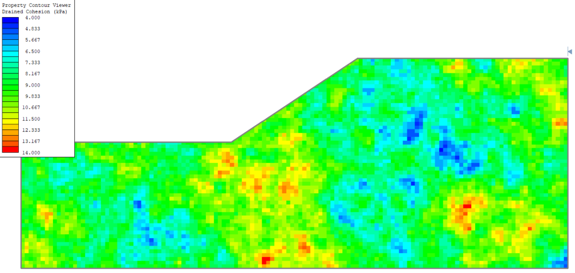
Conditional random field generated with observed borehole data. The top image shows a field with small correlation lengths, leaving most of the field unconditioned. The bottom image shows a field with larger correlation lengths, displaying the influence of the observed borehole data.
Slide2 conditions a field using Kriging – a methodology to find the Best Unbiased Linear Estimate (BLUE) of a desired point/cell in a field considering available observed data.
Linear Detrending
Borehole data typically increase with depth due to increasing overburden stress. This means the data is non-stationary (the mean changes with position/depth). Random field theory and Kriging assume stationarity, meaning we should ideally detrend the data before applying this data for conditioning.
Detrending the data involves 2 steps:
Use a common linear regression analysis, such as Ordinary Least Squares (OLS), to fit the observed data. For a linear fit:
Y = a + bx
where Y is the predicted value of the observed value y at x, b is the slope of the line, and a is the y intercept.
Detrend and standardize the observation at depth z:
Valz,detrended = (Valz - Y)/σr
where Valz is the observed value at depth z, and σr is the residual standard deviation of the observations determined by calculating the standard deviation of all Valz-Y at each depth.
This automatic detrending and standardizing process assumes a linear trend and that the observations are normally distributed. Furthermore, at least 3 observations within a grouping are required to have a meaningful linear regression analysis. If less than 3 observations exist, the observations for this group will be standard normalized without detrending.
Kiriging Estimation
Kriging estimation is used to condition the field. Fenton and Griffiths (2008) represent the Kriged estimate of  of the field
 with the following equation:

where x is the point of interest, n is the number of observations, βk are the weights multiplied by the observed values in the field Xk. The weights are dependent on the point of interest and reflect their relationship with location x.
These weights are solved by the equation

where K is the covariance matrix, populated by the covariances between all known points and observed points, and M is a vector of covariances between the point of interest and observed points.
Conditioning-By-Kriging
The final conditioned random field is created by finding the Kriged estimate of each cell in the field. This Kriged estimate is found using the following equation from Fenton and Griffiths (2008):
Zc(x)=Zu(x)+[Zk(x)-Zs(x)]
where x is the point of interest, Zc(x) is the value of the conditioned field at x, Zu(x) is the unconditioned value at x, Zk(x) is the Kriged estimate of the value based on known observations at x, and Zx(x) is the Kriged estimate of the value based on unconditioned field values at x.
The overall process requires a generation of the unconditional random field, followed by solving the weights for each point, then calculating Zc(x). Doing so allows the conditioning of the field.
- It’s assumed that all observations are standard normal and apply to all materials within the field. However, materials will only be conditioned with observations located within their defined zone.
- Borehole data (e.g. CPT) vary by depth and are unable to prescribe specific material properties without additional relational models. Therefore, borehole readings are treated as defining a shared spatial trend within one material for all properties for conditioning. Each property retains its individual statistical properties (ex. Distribution, mean, standard deviation) and correlations between other properties, but the influence of the borehole observations is shared between properties of the same material.
- Due to implying trends and conditioning using only observations within a material, it is essential to model the material layers rather than relying on the implied trend suggested by the borehole readings. Modeling layers as accurately as possible with their own statistical properties encourages a truer representation of the final conditioned field.
Overview of steps for conditional random field analysis
The general procedure for using conditional random fields in Slide2 is as follows.
- Select Project Settings > Statistics > Probabilistic Analysis, and select the Spatial Variability Analysis checkbox. Then select the Condition Random Field checkbox.
Define CPT Data by selecting Properties > Modify CPTs.
The Modify CPTs menu item will be disabled unless Condition Random Field is enabled and an external is defined.
- Preview the generated fields in the Property Viewer to ensure the field has been correctly defined.
- When you select Compute, the Overall Slope probabilistic analysis method is used. In general, this type of analysis will be longer than a typical Slide2 analysis, due to the repetition of the critical slip surface search required by the Overall Slope analysis.
- When you view results in Interpret, the presentation of results is mostly the same as for a non-spatial probabilistic analysis, with additional features of the Property Viewer.
- The Property Viewer option allows you to view the actual conditioned random fields generated by the analysis. This option is available in both the Slide2 Model and Interpret programs. In the Interpret program, you can view conditional random fields and results (slip surfaces) on the same plot, allowing you to see the effect of changing the conditioned random fields on the analysis results.
References
Fenton, G. A., & Griffiths, D. V. (2008). Risk Assessment in Geotechnical Engineering. John Wiley & Sons, Hoboken, New Jersey.onlinelibrary.wiley
Lloret Cabot, M., Hicks, M. A., & van den Eijnden, A. P. (2012). “Investigation of the reduction in uncertainty due to soil variability when conditioning a random field using Kriging.” Géotechnique Letters, Vol. 2, No. 3, pp. 123–127.