Spatial Variability
Spatial Variability Analysis is a sub-option of the Probabilistic Analysis in Slide2, which allows you to simulate the variability of soil properties such as strength and unit weight, with location within a soil mass.
What is spatial variability analysis?
Most real soil materials have properties which vary, to some extent, with the location within the soil mass. A traditional probabilistic slope stability analysis does not account for this type of variability. In a traditional probabilistic analysis:
- a statistical distribution is defined for a parameter (e.g. cohesion)
- for each simulation, the entire soil mass is assigned a single random value
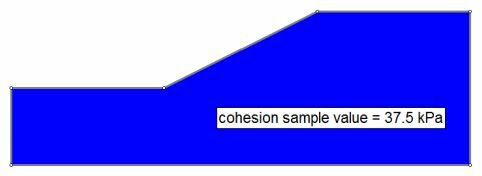
Single random sample value (cohesion) applied to the entire soil region
With spatial variability analysis:
- a statistical distribution is defined for a parameter
- correlation lengths are defined in the x and y directions
- for each simulation, a random field of values is generated for the soil mass
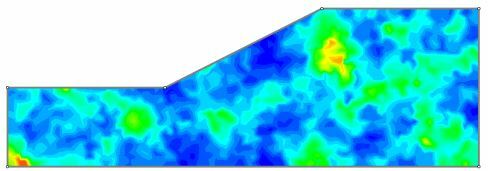
With spatial variability, rather than assigning a single randomly generated sample value to a soil region, a random field of values is generated for each sampling based on the statistical distribution and the correlation length parameters of a material. This creates a spatial distribution of values (e.g. cohesion) throughout the material, for each sampling, as shown in the above figure.
During the slope stability analysis, any slip surface which passes through a spatially variable material will encounter variability of properties along the slip surface.
Why use spatial variability analysis?
The premise of using spatial variability analysis is that real soil materials have properties which vary with location throughout the material. Therefore, an analysis which tries to account for this type of variability should provide a more realistic assessment of the mean factor of safety and probability of failure of a slope.
The use of spatially variable analysis has been shown to affect the calculated probability of failure of slope models. For example, it has been shown that for slope models with a mean factor of safety greater than 1, accounting for spatial variability of material properties (e.g. cohesion and unit weight) results in a LOWER probability of failure, compared to the same analysis without using spatial variability (Javankhoshdel et al., 2017). A probabilistic analysis that does not consider spatial variability has been shown to result in unrealistic and overly conservative probabilities of failure.
Overview of steps for spatial variability analysis
The general procedure for using spatial variability in Slide2 is as follows.
- Select Project Settings > Statistics > Probabilistic Analysis, and select the Spatial Variability Analysis checkbox. See the bottom of this page for information on the Covariance Function and Mesh Size option.The Overall Slope Analysis Type is automatically selected. Due to the nature of a spatial variability analysis, you must use the Overall Slope probabilistic analysis type since a new random field is generated with each sample for each spatial material.
- In the Material or Hydraulic Statistics dialog, define the Correlation Lengths in the X and Y direction for each material you are defining as spatially variable.Correlation lengths are defined per material.
- Preview the generated fields in the Property Viewer to ensure the field has been correctly defined.
- When you select Compute, the Overall Slope probabilistic analysis method is used. In general, this type of analysis will be longer than a typical Slide2 analysis, due to the repetition of the critical slip surface search required by the Overall Slope analysis.
- When you view results in Interpret, the presentation of results is mostly the same as for a non-spatial probabilistic analysis, with additional features of the Property Viewer.
- The Property Viewer option allows you to view the actual random fields generated by the analysis. This option is available in both the Slide2 Model and Interpret programs. In the Interpret program, you can view random fields and results (slip surfaces) on the same plot, allowing you to see the effect of changing random fields on the analysis results.
Covariance Function
Three covariance functions are available with spatial variability: Markovian, Markovian 1D Separable, and Gaussian. During the random field generation using the Local Average Subdivision method, the covariance functions are used to calculate the covariance value between cells in the field. This is where the correlation length input (see section below) is taken into account. Each method uses a different equation to model the reduction of covariance with distance.
- Markovian: covariance = variance * exp( -tau ), where tau = sqrt[ (2*X/CLX)^2 + (2*Y/ CLY)^2 ]
- Markovian 1D Separable: covariance = variance * rX * rY, where rX = exp(-2|X|/CLX), rY = exp(-2|Y|/CLY)
- Gaussian: covariance = variance * rX*rY, where rX = exp( -pi*(X/CLX)^2 ), rY = exp( -pi*(Y/CLY)^2 )
Automatically Calculate Mesh Size
The mesh size in a random field must meet two requirements: 1) it is recommended that it be at least half of the smaller correlation length (X or Y), and 2) each material layer must have a sufficient amount of cells to correctly represent the variability (for example a thin horizontal layer should not have just one row of cells because this would not take into account the vertical variability). Slide2 uses an algorithm that automatically calculates the mesh size for each layer in order to satisfy these requirements. It is recommended that this checkbox is not turned off. However, the user may turn off the checkbox if they want to define their own mesh size for spatially variable materials.
Analysis Type
Due to the nature of a spatially variable probabilistic analysis, you must use the Overall Slope Analysis Type option. This is because for each sampling a new random field of material properties is generated for the spatially variable materials. Therefore the critical slip surface search must be repeated for each new random field.
Properties Available for Spatial Analysis
At present the spatial variability analysis in Slide2 only works in conjunction with the following strength models:
- Mohr-Coulomb
- Undrained (constant or linearly increasing)
And the following material parameters:
- Cohesion
- Friction Angle
- Unit Weight
- Shear strength (COV method)
And the following parameters for hydraulic statistics:
- Saturated Permeability
- Saturated Water Content
- Residual Water Content
Note that any randomly defined variables not included in the above list will be removed if spatial variability option is turned on.
Spatial variability cannot be applied to any other material parameters.
Number of samples & sampling method
For spatial variability analysis, a large number of samples, and the Latin Hypercube sampling method is recommended. A minimum of 1000 samples should be used or higher (e.g. 2000 to 10,000 depending on the model complexity).
The Number of Samples is specified in Project Settings > Statistics.
Number of slices
For spatial variability analysis, it is not necessary to increase the number of slices from the default. Slide2 uses a sub-sampling method to sample the bottom of each slice, and hence properly sample all the cells at the bottom of each slice.
Correlation Length
The Correlation Length represents the distance within a material over which values of a spatially random variable (e.g. cohesion) are expected to be highly correlated (i.e. similar in magnitude). In practice, two samples taken from adjacent locations in the soil profile tend to have very close values and as the sampling distance increases this tendency decreases. Small values of spatial correlation length mean that soil properties highly fluctuate; on the other hand, large values of spatial correlation length mean that soil properties vary smoothly within the soil profile. If the Correlation lengths are equal in the X and Y directions, this will generate isotropic random fields (i.e. no preferred direction, same spatial variability in the horizontal and vertical directions).
Spatial Variability Tutorial
After you have enabled spatial variability analysis in Project Settings, you must define correlation lengths for your spatially variable materials in the Material Statistics or Hydraulic Statistics dialog. For an overview of Spatial Variability Analysis in Slide2 and a step-by-step tutorial example, see Tutorial 10 - Spatial Variability.