Interpolation Method

There are many different methods which can be used to interpolate values from a grid of data specified at X and Y locations. Interpolation implies that the value of a variable can be determined at any required location, based on the defined values at specified locations.

In Slide2, Interpolation Methods are used for:

• Interpolating values of pore pressure, if the Groundwater Method in Project Settings, is set to one of the three available Water Pressure Grid methods – Grid (Total Head), Grid (Pressure Head), Grid (Pore Pressure). See the Groundwater Method topic for details.
• Interpolating values of shear strength parameters (cohesion, friction angle), if the shear strength of a material in the Define Material Properties dialog, has been specified using the Discrete Strength Function option. See the Discrete Strength Function topic for details.
• Interpolating soil profile boundaries from borehole data.

The following Interpolation Methods are available in Slide2.

Thin Plate Spline

The Thin-Plate Spline method utilizes the concept of an infinite thin elastic plate under tension, to determine a spline surface (a smooth 3-dimensional surface which fits through all of the data points). The spline surface is used to determine the sample value at any location (Franke, 1985).

Chugh’s Method

This is an interpolation method based on finding the nearest grid point, in each of the four quadrants with origin centered at the point where the interpolation is required (e.g. at the midpoint of the base of a slice). A plane is then fit through each combination of three quadrant grid points, and interpolation is performed for each plane. This results in four interpolations, which are then averaged to obtain the final interpolated value at the desired point (Chugh, 1981).

Modified Chugh

This is based on the Chugh method, with the additional requirement that the interpolation point must be WITHIN the triangle formed by any combination of three quadrant points. If the interpolation point is NOT within a triangle, then this combination of quadrant points is NOT used. This check ensures that EXTRAPOLATED values are not included in the average interpolated value. This avoids numerical inaccuracies which sometimes occur with the Chugh method, due to excessively large extrapolated values.

Local Thin Plate Spline

The Local Thin-Plate Spline method is an extension of the Thin-Plate Spline interpolation technique and is recommended for use with a large number of data points (>200). The only difference between the methods is that instead of using all the data points for the interpolation, the Local version takes a maximum of 10 closest points to the sample point and fits a spline surface through them. The local spline surface is then used to determine the sample value.

TIN Triangulation

TIN Triangulation (Triangulated Irregular Network) takes the data points and triangulates them using the Delaunay triangulation method. To calculate the value at a sample point, the program first determines which triangle the point lies within. Once the triangle that contains the sample point is found, the interpolated value is calculated using linear interpolation. This is done by calculating the plane equation that fits through the 3 data points at the triangle vertices, then solving for the value using the coordinates of the sample point and the plane equation.

Inverse Distance

The Inverse Distance Interpolation method weights every data point according to its distance to the sample point. This scheme is also known as the Shepard method (Shepard, 1968) and can be written in the form:

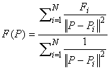
where P is the location of the point to be interpolated, F(P) is the interpolated value, Pi the location of the scattered data, Fi are the scattered data values, and ||P-Pi||2 represents the distance from P to Pi. The main deficiencies of this method are: 1) the local extrema are typically located at the data points and this results in poor shape properties, and 2) undue influence of points which are far away from the sample point.

Linear By Elevation

The Linear by Elevation method only utilizes the elevation (y-coordinate) of each data point. The method simply determines the closest data point (elevation) above the sample point and the closest data point (elevation) below the sample point and linearly interpolates the sample value based on these two data points. Interpolation is done in the vertical direction only. This method is meant for horizontally bedded soils where data varies by depth only. It is extremely useful for cases where a complicated strength or pore pressure profile exists in only the vertical direction. The x-coordinate of the data points is not used in the interpolation process. However, it is used to display the data on your model.

Kriging

Kriging is a best linear unbiased estimator (BLUE), or a weighted average that minimizes the prediction error associated with the estimate. Ordinary Kriging is used in Slide2, meaning that the mean is assumed to be constant but unknown. The weighted average equation is expressed as follows:

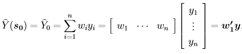
Where y is the vector of sampled values, and w’ is the vector of weights applied to the sampled values. The weights are based on the covariances between the sampled points, and the covariances between the sampled points and the point to be predicted. Slide2 uses an exponential semivariogram for estimating the covariances. For compatibility with a large number of data points, the kriging method takes a maximum of 50 closest points to the point to be predicted.

Reference:

Bailey, Trevor and Gatrell, Anthony (1995). “Ordinary Kriging.” Interactive spatial data analysis. Longman Scientific & Technical, New York, Ch.5.5

Secondary Interpolation Method

Because cases exist where interpolation at a sample point cannot be performed, backup methods are used if the initial selected method fails.

• If Local Thin-Plate Spline fails, then Inverse Distance is used instead.
• If any of the other methods fail, the Local Thin-Plate Spline method is used.

Display of Interpolation Contours

In the Slide2 Interpret program, contours of the approximate results of the interpolation process can be displayed on the model, by selecting the Supplemental Contours option in the Data menu.

The interpolation results should always be looked at to ensure that the interpolation correctly simulates your field data. If it does not, then either more data points should be used or a different interpolation technique. Since no interpolation method is guaranteed to work for all datasets, different methods should be tried in order to determine the best method for your data.