10 - Spatial Variability

1.0 Introduction

This tutorial example will demonstrate spatial variability analysis involving a multi-material rock-faced tailings dam model (Ref.1). We will compare the results of the model with and without spatial variability.

We will demonstrate how to:

• Assign spatially variable properties to materials
• View contours of spatially variable properties
• View results for specific realizations from the set of statistical simulations

For an overview of Spatial Variability Analysis in Slide2, see Spatial Variability.

The finished product of this tutorial can be found in the Tutorial 10 Spatial Variability.slmd data file. All tutorial files installed with Slide2 can be accessed by selecting File > Recent Folders > Tutorials Folder from the Slide2 main menu.

2.0 Model Geometry

1. Select File > Recent > Tutorials and open Tutorial 10 Spatial Variability – starting file.slmd.


Notice in the Document Viewer that the model has three scenarios already defined. The master scenario is deterministic, whereas the two child scenarios will contain the non-spatial and spatial analysis, as named.

The model has five different materials. The type of material and corresponding properties is already defined in the starting file and are as shown on the Material Properties dialog image below. To open the Material Properties dialog:

2. Select Properties > Define Materials
   

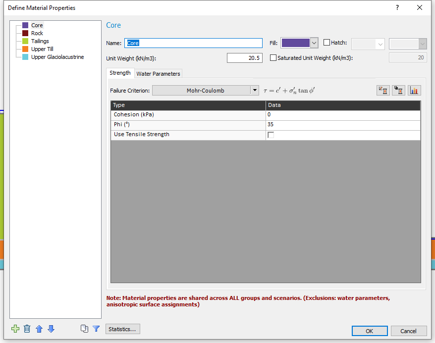
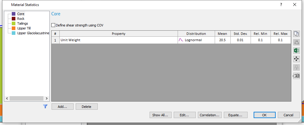
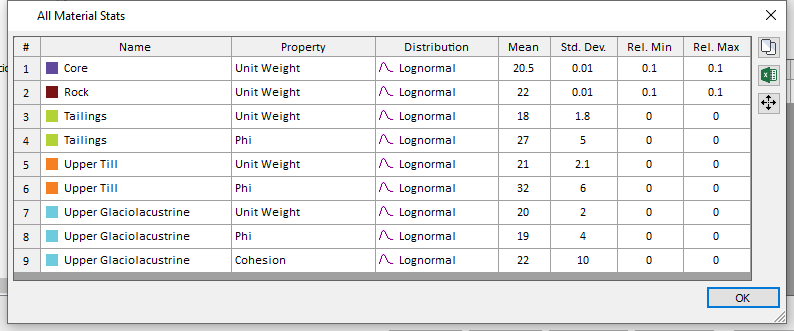
Statistical distributions have also been defined for the slope materials.

• Unit weight is a random variable for all five materials.
• Friction angle (Phi) is a random variable for the Tailings, Upper Till and Upper Glaciolacustrine materials.
• Cohesion is a random variable for only the Upper Glaciolacustrine.

To view the statistical parameters:

3. Click on the Statistics button to open the statistical distribution table.
   
4. Click on Show All in the Material Statistics dialog to view all the random parameters defined.
   
5. Click OK to close the ‘All Material Stats’ dialog and select Cancel on the remaining dialogs.

3.0 Setting up the Spatial Analysis

We will now set up our Spatial Analysis in the last scenario.

1. Select the Spatial Variability Scenario.
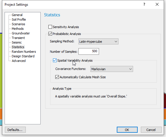
2. Select Analysis > Project Settings
3. Select the Statistics tab and tick the checkbox beside the Spatially Variability Analysis as shown below.
4. Click OK to close the dialog.

For this tutorial, we will define spatially variable material properties for the Tailings, Upper Till and Upper Glaciolacustrine. To do this, we must input correlation length parameters for these materials.

The correlation length parameters for all the spatially variable materials are assumed to be 20m in the x and y directions.

1. Select Statistics > Materials
   
2. Select the Tailings material and tick the checkbox beside the Spatially Variable Material.
3. Enter a Correlation Length of 20 m for both X and Y directions.
   
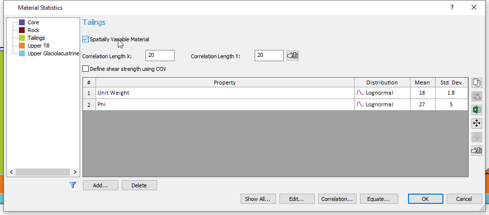If you are unsure about what correlation length values to use, the button next to the "Correlation Length Y" field will open up a table from the literature that summarizes correlation length values for different types of soils.
4. Repeat steps (2) and (3) for the Upper Till and Upper Glaciolacustrine layers.
5. Click OK to close dialog.


Before computing, we can preview the spatial fields we have defined using the Property Viewer.

6. Select Analysis > Property Viewer
   
7. On the left side, set the Property to Unit Weight, and set the Filter to “Show Variable Only” in order to view only the spatial materials.
   
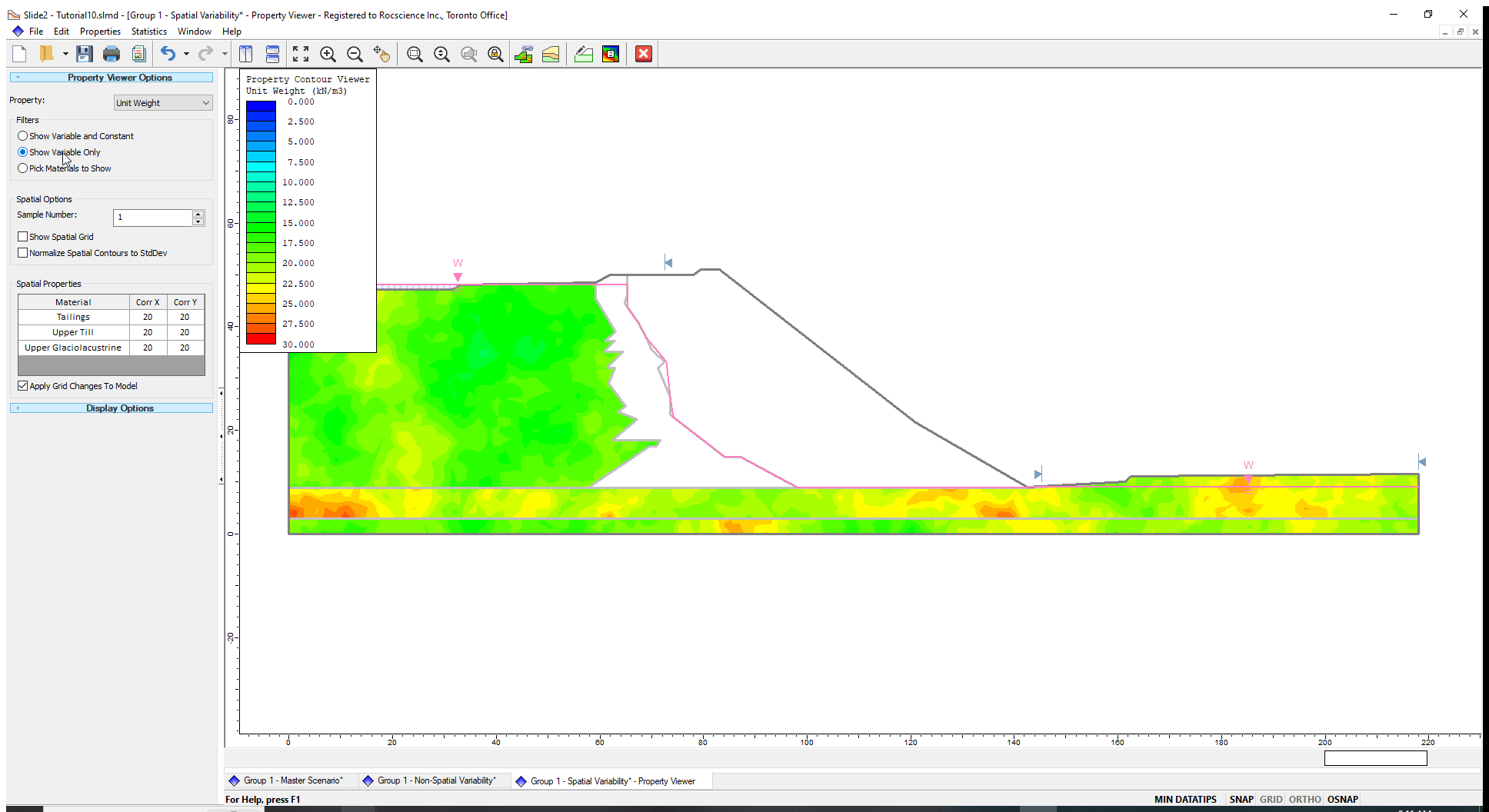
8. Click the up arrow next to Sample Number to flip through the 500 simulations of the unit weight random field. You can also play around with different values of correlation length and see their impact on the field live. See the Property Viewer page for more details.

Now, we will compute both Scenarios using non-circular slip surfaces with surface altering optimization. The GLE/Morgenstern-Price limit equilibrium method is used in this model (as can be seen in the Methods tab of Project Settings).

4.0 Computation and Interpretation

1. Select Analysis > Compute . This analysis will take approximately thirty (30) minutes to compute.
2. Select Analysis > Interpret to view the results when the computations are done.

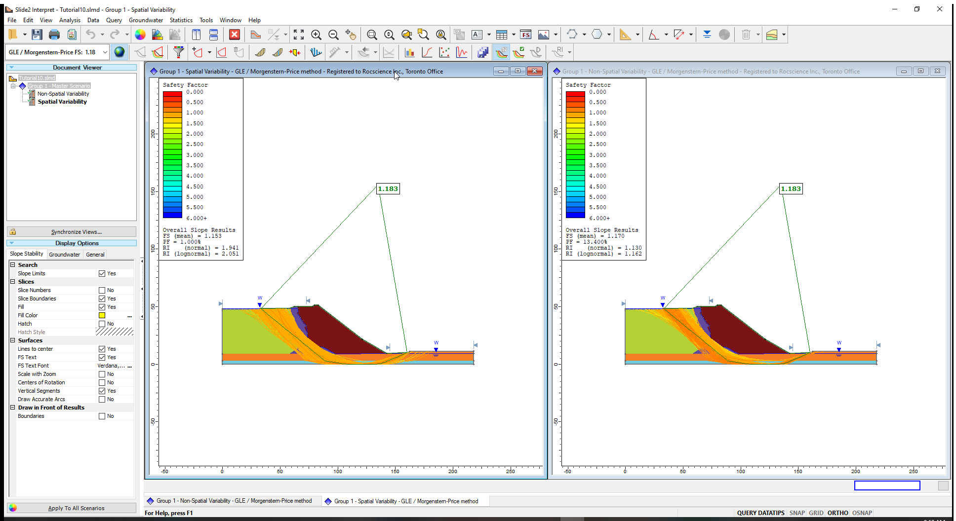
As expected, the deterministic FS and slip surface are the same for both scenarios. The result of interest is that with the spatial variability included, as the probability of failure reduces from 13% to 1%.

Let us view the safety factor distribution for the two scenarios:

1. Select Statistics > Histogram .
2. In the Histogram Plot dialog, choose Data to Plot = Factor of Safety.
3. Tick the Highlight Data checkbox and select Factor of Safety < 1 .
4. Click Plot to create the histogram.
5. Do this for both the spatial and non-spatial scenarios.
6. Select Window > Tile Windows Vertically and minimize the necessary scenarios until you have the non-spatial histogram on the left and spatial histogram on the right, as shown.

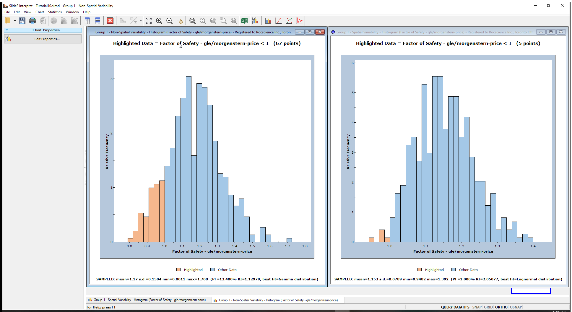
From the legend on the chart, the highlighted or (light brown) bars indicate the points with FS<1. Other FS statistics are also displayed below the chart.

From the histograms, we can conclude the following:

1. The distribution of safety factors from the overall slope probabilistic analysis with spatial variability is much narrower than the analysis without spatial variability. (Notice the range of FS in the histogram on the left compared to the range of FS in the histogram on the right.)
2. With spatial variability included, fewer slip surfaces had FS < 1, resulting in a lower Probability of Failure. These outcomes show that considering spatial variability reduces the probability of failure (or the risk).

5.0 Property Viewer

The Property Viewer is available in both the Modeller and Interpreter programs. In Interpret, the Property Viewer can show results for slip surfaces corresponding to the individual realizations (simulations) of the spatial probabilistic analysis.

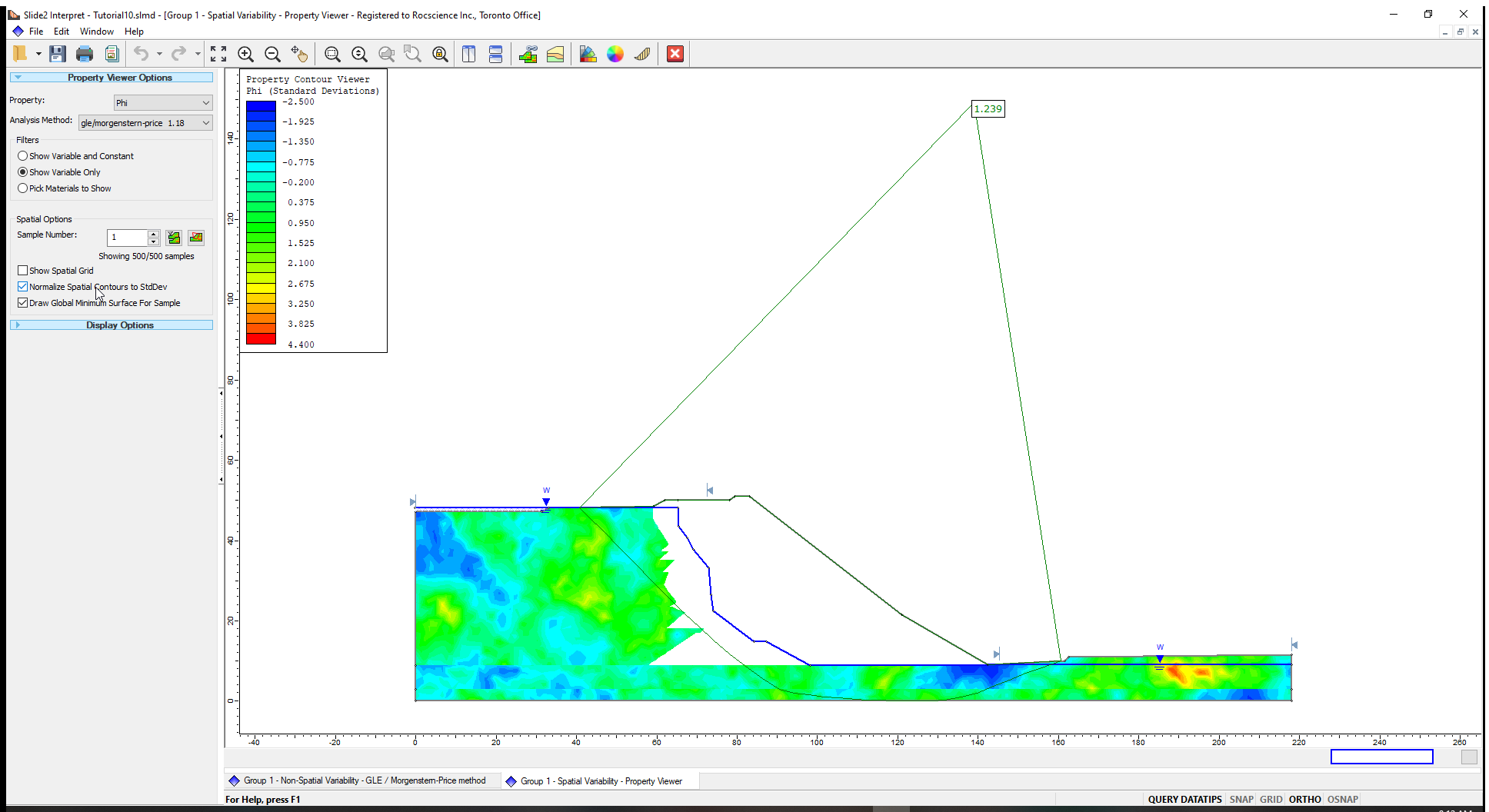
Let us view the Phi contours for the spatially variable slope materials.

1. In the Slide2 Interpret window, maximize the ‘Spatial Variability’ results and select Analysis > Property Viewer
   
2. In the Property Viewer Options in the sidebar, select the following parameters:
• Property = Phi
• Analysis Method = gle/morgenstern-price (method selected in Project Settings.)
• Filters = Show Variable Only (This means we will see only the contours of the spatially variable material).
3. Tick the checkbox for Normalize Spatial Contours to StdDev.

The ‘Normalize Spatial Contours to StdDev’ option standardises the contours for each spatially variable material, relative to its standard deviation. This plot helps you to quickly see the relative minimum and maximum values of the different random fields.

As you scroll through the sample numbers (simulations), you will notice the display of the global minimum slip surface corresponding for the current sample.

The Phi contours for the spatially variable materials (Till, Upper Till and Upper Glaciolacustrine) and the Global Minimum slip surface for Sample Number (1) is shown below.

There are two icons to the right of the Sample Number field.

• Filter Samples is used to filter samples that can be viewed.
• Minimum Factor of Safety is used to show samples that give the minimum factors of safety.

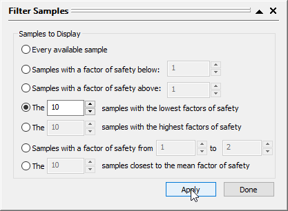
Let us view the ten (10) realizations that produced the lowest factors of safety in the analysis.

1. Click on Filter Samples to open the ‘Filter Samples’ dialog.
2. Select the option of Samples with the lowest factors of safety and enter 10.
3. Click Apply.
4. Click Done to close the dialog.
   
   
   
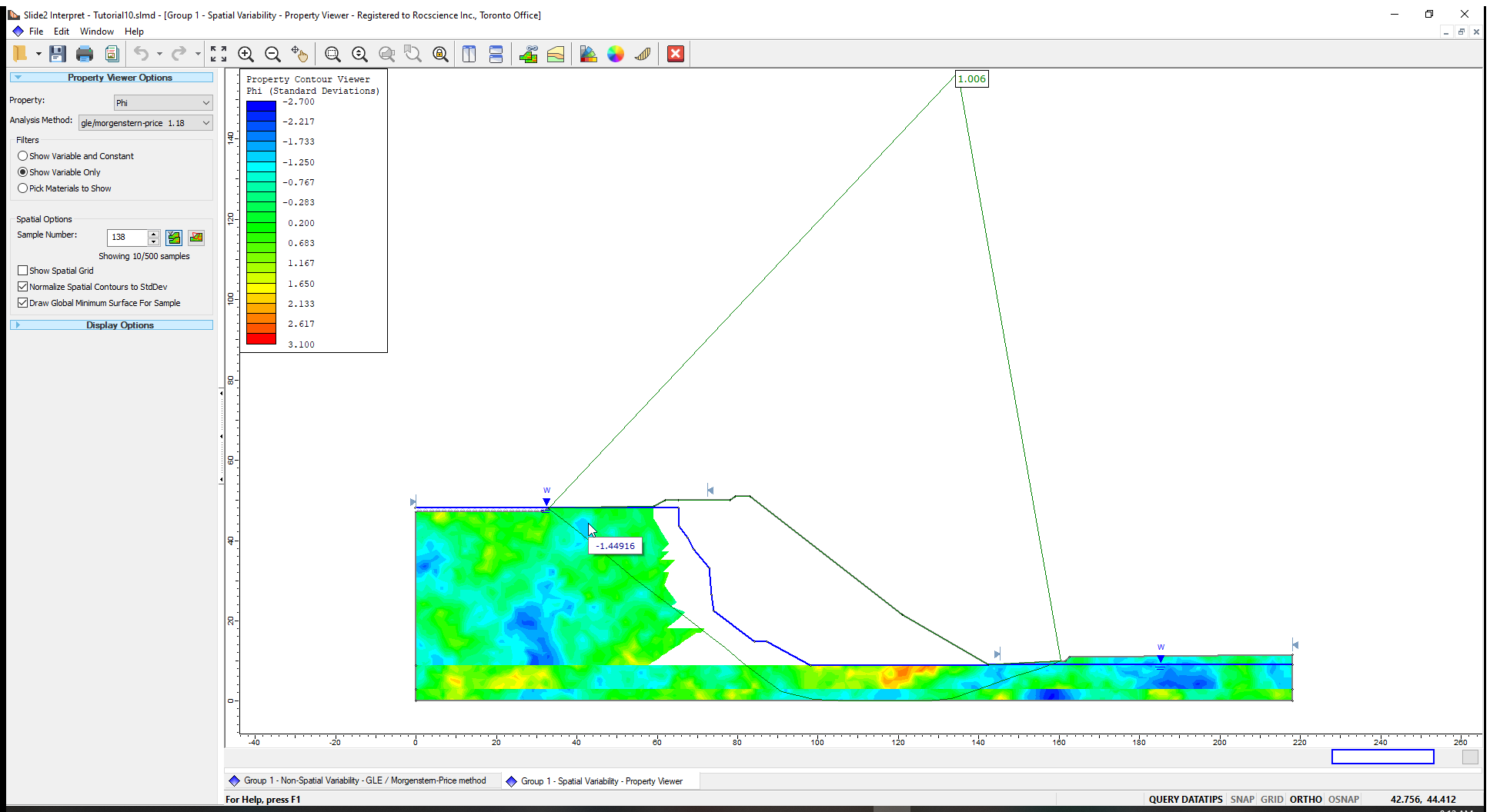
5. Place the mouse on the Sample Number field in the sidebar and scroll through the sample numbers in the sidebar.

You will see that only the 10 lowest safety factor samples and slip surfaces are displayed on the model.

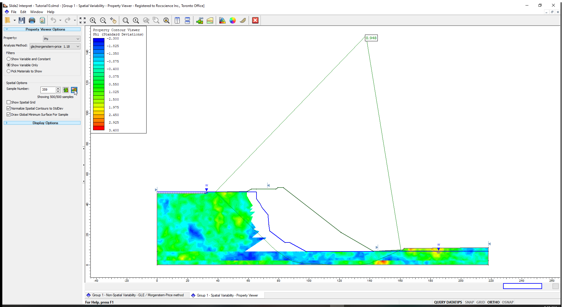
Now we can find the minimum safety factor out of the ten (10) lowest safety factors filtered.

1. Click on the Minimum factor of safety button.
2. The Sample Number shown in the box has the minimum factor of safety as shown below.

This concludes the tutorial.

You are encouraged to experiment with the Property Viewer Options and the Contour Options to become more familiar with the many different display options.

For more information about Property Viewer options, check out the Property Viewer help page.

6.0 References

Cami, B., Javankhoshdel, S., Lam, J., Bathurst, R.J. and Yacoub, T. 2017. Probabilistic analysis of a tailings dam using 2D composite circular and non-circular deterministic analysis, SRV approach, and RLEM. 70th Canadian Geotechnical Conference, Ottawa, Ontario, 7 p.