Weak Layer Overview
The Weak Layer option allows you to define a surface with its own material properties. This can be used to model any type of joint, discontinuity or interface along which failure might occur.
There are two options available to define a Weak Layer surface:
See Multiple Weak Layers Tutorial for examples of how to use the Weak Layer options.
How weak layers work in Slide3
If there are weak layers in the model and they intersect a slip surface generated during the search (or user-defined surfaces), then the following options (available via Slip Surface Options > Weak Layer Handling) will determine the logic for clipping the slip surfaces to the weak layers:
- Always snap to highest layer – An envelope of weak layers will be used to clip the slip surface. More specifically, if an active weak layer exists above any given point on a slip surface, then the elevation of the slip surface will snap to the highest weak layer at that location.
- Automatic case generation – For a given slip surface and the weak layers that it touches, the program will determine all applicable combinations of toggling each weak layer on and off and attempt to evaluate the factor of safety for each case. Note that for models with many weak layers, this option may slow down the search significantly.
- Heuristic – Toggles the weak layers on and off during the random search process (available only for Particle Swarm Optimization and adapted from Kennedy and Eberhart (1997)). Weak layers producing lower factors of safety tend to remain toggled more often as the search progresses. It is much more efficient than the Automatic case generation for models with many weak layers.
See Multiple Weak Layers Tutorial for a demonstration of how these options can be used. Some additional details about the logic for clipping slip surfaces to the weak layers are discussed below.
Entire weak layer
Note that each weak layer defined in a model is assumed to exist in its entirety. Slip surfaces affected by the weak layer are either cut by the entire weak layer or, when considering the various cases during automatic case generation, not cut at all.
Suppress weak layer
It is possible to completely exclude a weak layer defined in the model from the analysis, without having to delete it. You can do this by checking off the “Suppress” checkbox in the weak layer properties.
Discontinuous layers
If a weak layer enters a given slip mass but does not fully exit the mass, either via the ground surface or through the slip surface, then it is discontinuous.
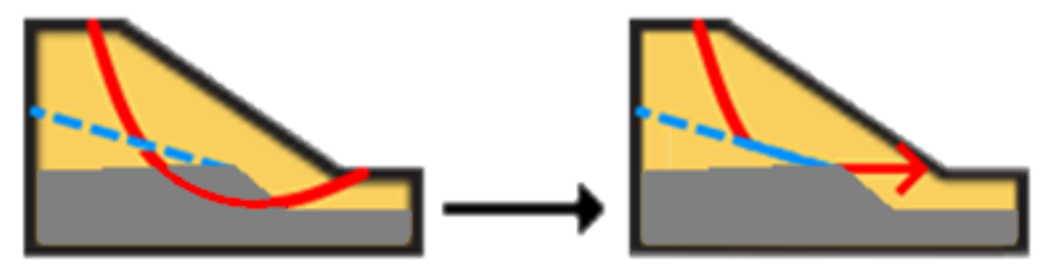
Discontinuous weak layers can significantly increase the difficulty of the search routine for finding the critical slip surface. For example, the image shows a blue weak layer that ends inside of a slip mass (delineated by the red line) near the ground surface.
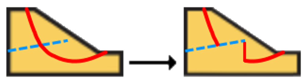
The discretization process will initially snap the portion of the slip surface found below this weak layer up to the weak layer. In Slide2, the rest of the slip surface will not be changed, resulting in a slip surface with a local discontinuity which may render it invalid. However, for Slide3 an extrapolation scheme described in the following section will be attempted to produce a valid surface.
Horizontal extrapolation
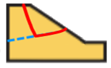
For the above example, Slide2 will discard the slip surface with the local discontinuity shown, because it is relatively easy to generate a better slip surface such as the one shown in the following image. This is because in Slide2, slip surfaces can be drawn using simple polylines or circular arcs.
However, in Slide3, the geometrical parameters defining the slip surfaces are much more complicated. For this reason, it can sometimes be helpful to apply an extrapolation of the discontinuous layer to cut the slip surface beyond the extents of the weak layer, as shown in the figure below.
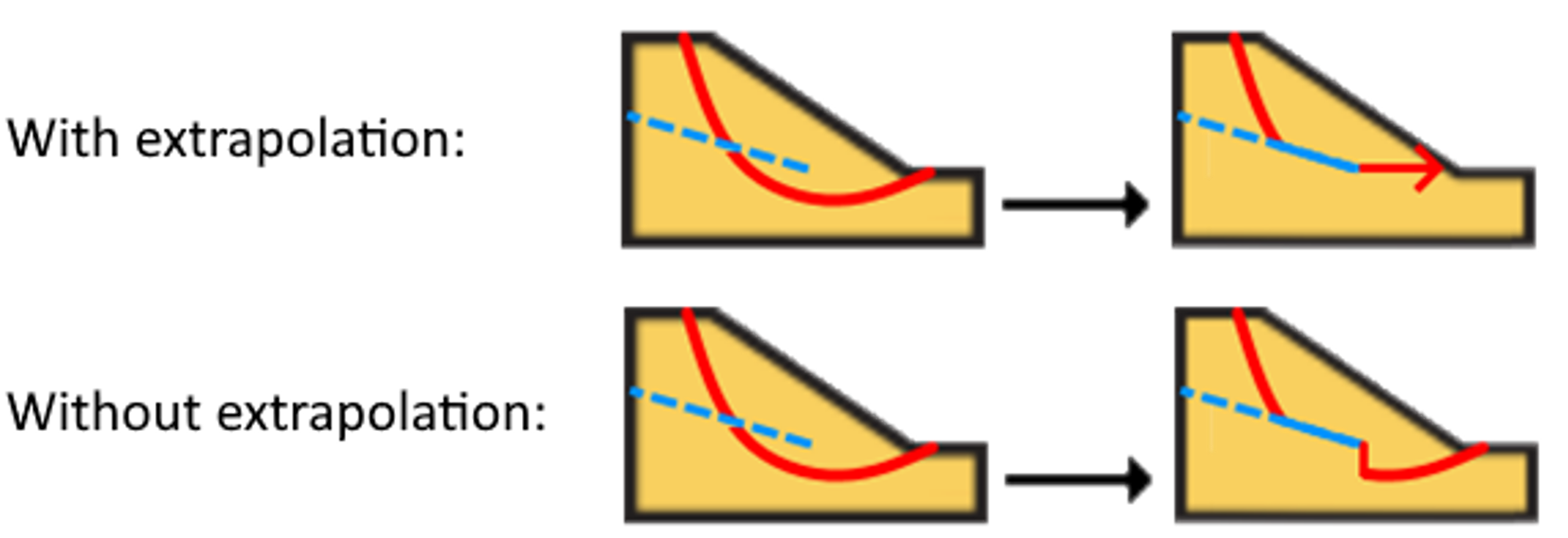
To help visualize this, a few examples of how this logic is applied are shown below.
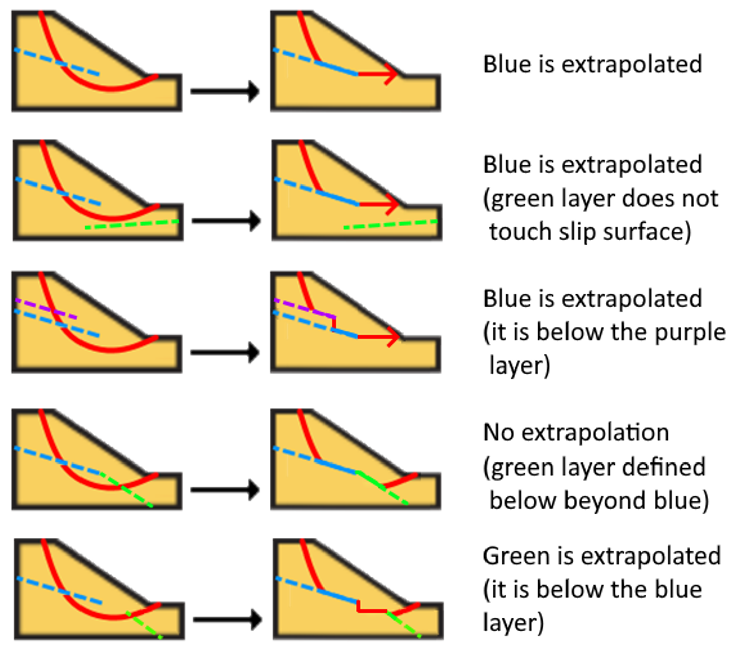
Note that weak layers deactivated for a given case during the automatic case or heuristic case generation will not be considered during the extrapolation. The above examples only show cases where the visible weak layers are all active. For example, if the green layers were deactivated during weak layer handling, the end of the blue layer will be extrapolated horizontally.
Finally, please be advised that the extrapolation of discontinuous weak layers may cause material blocks beneath the extrapolation to be ignored in the analysis. For example, the grey layer in the example below will be missed due to the extrapolation.
The grey layer will only be analyzed for the case where the blue weak layer is not considered (i.e. during automatic case generation).
Results naming
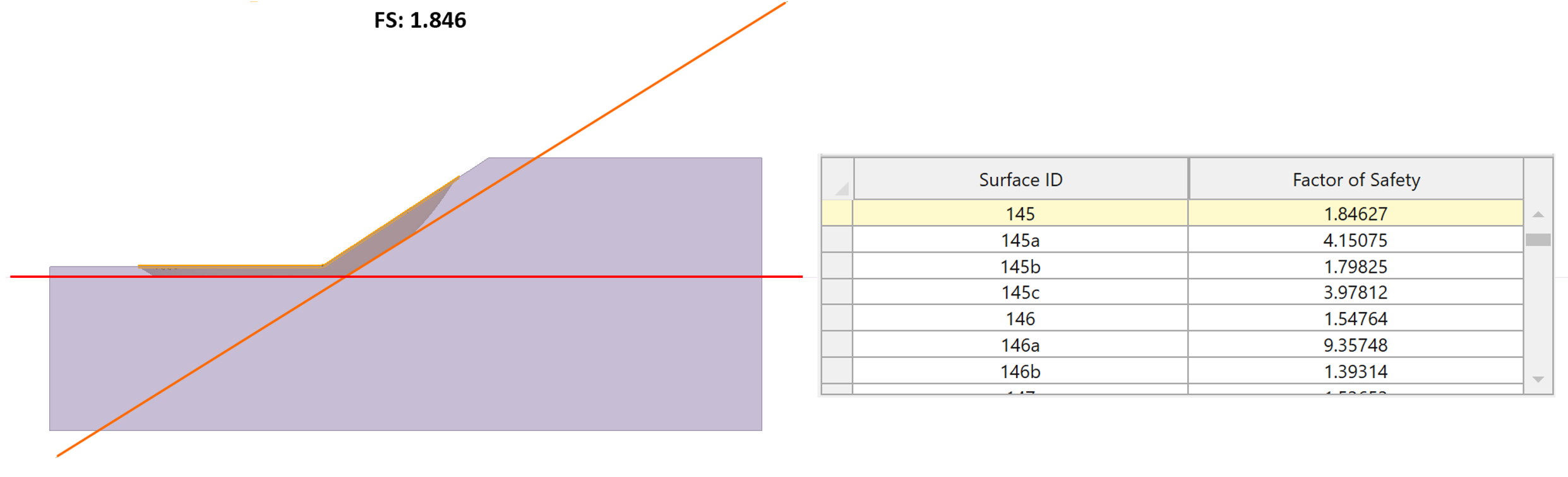
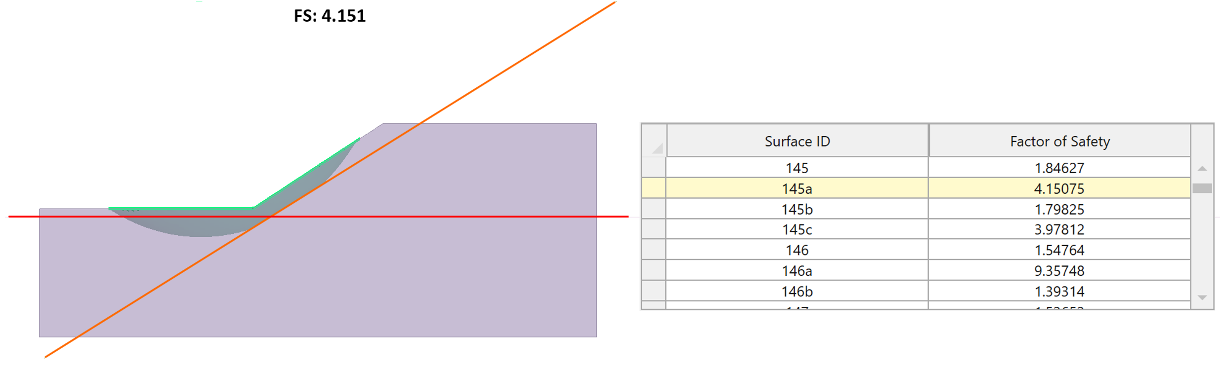
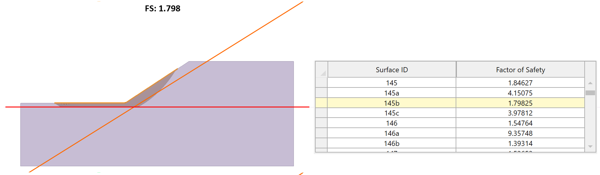
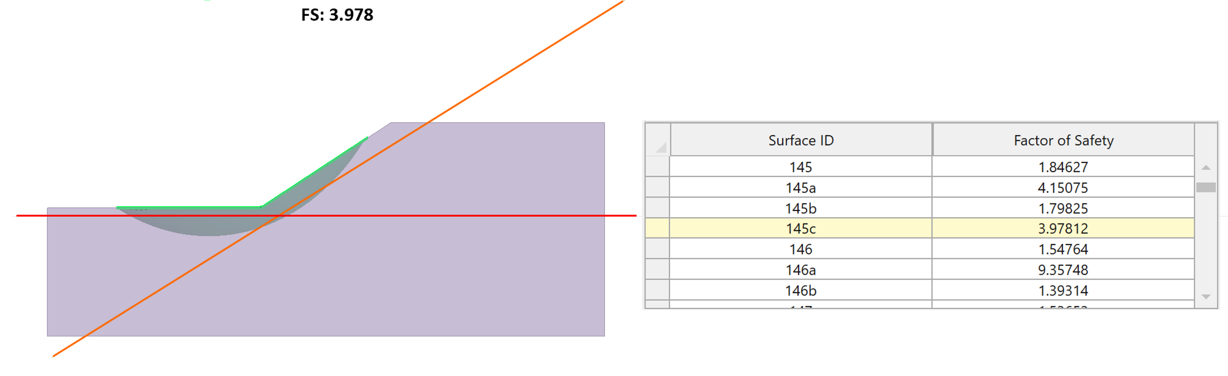
For a given user-defined slip surface that intersects multiple weak layers, there will be several cases evaluated if Automatic Case Generation is selected. This will produce multiple slip surfaces, which if they converge, will show up in the Show All Surfaces interface with suffixes a, b, c, etc.
Weak Layer Intersection with Ground
If the weak layer intersects the ground surface continuously throughout the slipping mass so that it produces a clean cut, then the portion of the slip mass outside of the cut will be discarded. If it is not a clean cut, then the slip surface will likely be discarded.
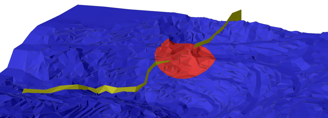
An example of a clean cut with a weak layer through the ground surface in a spherical slip mass is shown below. The entire weak layer protrudes the ground surface and clips the slip surface.
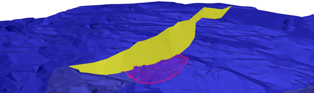
The following image shows a yellow weak layer that only partially protrudes the ground surface in the region of the red slip sliding surface – such a surface will not be admitted in the analysis.
Vertical and Near-Vertical Weak Layers
Slide attempts to cut slip surfaces using the weak layers that they intersect. However, if the weak layers are vertical or near-vertical, there are many potential discretization issues which can occur. The logic of weak layers clipping the slip surface can be become complicated if they are present in the model. Some special cases involving these vertical and near-vertical weak layers are explained in the following sections.
Issue 1. Very Steep Column Bases
If a very steep weak layer is active and clips a slip surface, the resulting bases of the soil columns in that region will be very steep. Columns with very steep base angles are known to induce numerical instability in limit equilibrium methods and should be avoided if possible. In the following illustration, the slip surface is clipped by a steep vertical weak layer (weak layers are shown via dashed lines).
If the base angle of a column, θ, exceeds the maximum allowable angle, θmax, then the slip surface will be discarded with Error -413. The default value of θmax is 80°, which can be changed via Project Settings > Advanced).
Issue 2. Reverse Curvature
Very often, if any part of a weak layer is nearly vertical, there is a possibility that a part of it exhibits reverse-curvature. That is, a vertical line can be drawn to intersect the weak layer more than once, such as in the example shown below (illustrated in 2D for simplicity).
In this case, the slip surface would still attempt to snap to the highest point of the weak layer at any location. However, if the geometry of the weak layer is complex then the bottom of a slip surface at this region could become irregular, and the discretization of the slip surface will likely be unsuccessful.
Issue 3. Completely Vertical Weak Layers
Fundamentally, limit equilibrium cannot handle vertical cuts to slip surfaces. However, vertical cuts in slip surfaces can be valid if they are formed by tension cracks.
In only some specific cases, vertical weak layers can produce valid slip surfaces for analysis. Currently, Slide3 only considers vertical weak layers if they make a clean cut in the slipping mass completely up to the ground surface. Otherwise, it may not be detected and can introduce other discretization errors.
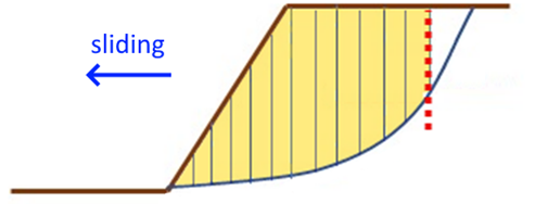
When vertical weak layers intersect the soil columns, they are treated similarly to tension cracks. These columns are removed from the analysis, and the neighboring exposed edges of soil columns are checked to see whether they are in compression with respect to the slip direction (defined below). Considering that vertical weak layers can split the slipping mass into one or more disjointed parts, the analysis will admit largest portion of the slipping mass which does not contain exposed column edges in compression.
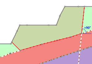
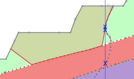
As an example, a vertical weak layer (red) is shown below, which splits the slipping mass into two regions. The sliding mass in the lower region is valid because the cut is made upslope from the mass with respect to the sliding direction. No reaction force is assumed to be exerted by the soil to the right side of the cut (it is assumed to be a zone of tension), and the material properties of the vertical weak layer are ignored.
However, the portion of the slipping mass upslope to the weak layer is invalid because the soil column which would be immediately to the right of the vertical weak layer has its exposed edge facing the weak layer in compression (a compressive reaction force can be expected from the interface touching the weak layer).
Note that in 3D, it is possible that for geometrically complex weak layers, regardless of the slip direction, the separate masses split by a vertical weak layer will become invalid because some columns at the intersection will be in compression. If this case is ever encountered, Slide will report Error -149 and prompt a warning when viewing the results.
Modelling Recommendations
If the user wishes to perform a slip surface analysis where it intersects a geometrically complicated weak layer with near-vertical and/or vertical portions, the following recommendations can be taken to increase the likelihood of getting a valid result:
- Ensure the weak layer protrudes through the ground surface completely.
- If there is reverse curvature in the weak layer, either manipulate its geometry to prevent reverse curvature or split it into multiple weak layers.
- If there are weak layers in the model which don’t appear to be oriented in the expected direction of sliding, consider just suppressing them from the analysis to improve performance and ease the search process.
- Remember that vertical weak layers usually only produce meaningful slip surfaces if they are generally aligned perpendicular to the sloping direction and are located near the crest of the slope.
- Consider using Tension Cracks instead of vertical weak layers if the intention is to truncate the crest of the slip surface.
- Use more advanced techniques such as finite element analysis in RS2 & RS3, which consider the behavior of the entire slope.
Warning messages
To warn the user about vertical or near-vertical weak layers or reverse curvature weak layers, two warning messages have been added to Slide3. For information about why vertical weak layers and reverse curvature can cause problems, see the section above.
Note that these warnings appear if at least 5% of the weak layer surface meets the criteria for vertical or reverse curvature. If your surface has these bad qualities in areas of the model in which you are not interested, you can safely ignore these errors.
The criteria is defined as follows:
- A weak layer is said to be near-vertical if at least 5% of the surface is inclined greater than 80° from the horizontal.
- A weak layer exhibits reverse curvature if at least 5% of the surface has points (x,y) with more than one z.
References
J. Kennedy and R. C. Eberhart, "A discrete binary version of the particle swarm algorithm," 1997, IEEE International Conference on Systems, Man, and Cybernetics. Computational Cybernetics and Simulation, 1997, pp. 4104-4108 vol.5, doi: 10.1109/ICSMC.1997.637339.