Layer Properties Overview
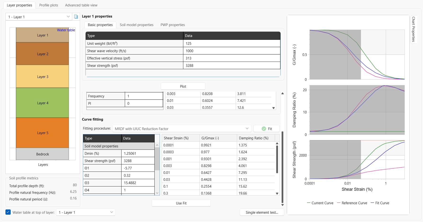
The Layer Properties tab allows the user to select layers, and define the properties of each layer of the soil profile (Thickness, Unit Weight, Shear Wave Velocity (VS) or Initial Shear Modulus (Gmax), etc.).
The Layer Properties tab is divided in several sections, some of which are only available depending on the Analysis Method selected:
- Basic Properties
- Soil Model Properties
- Pore Water Pressure (PWP) Properties (if applicable)
- Reference Curve (if applicable)
- Curve Fitting (if applicable)
On the right side of the window the plots of G/Gmax, Damping Ratio and Shear Strength vs Shear Strain are shown, with a Chart Properties pop out menu to adjust the display of the plots.
Select/Edit a Layer
The drop down menu at top left corner of the window can be used to
select the layer to view/edit. Alternatively, the user can click
on the layer they want to modify from the visual display on the left
side of the window.
Basic Properties
The basic properties tab includes the Unit weight, Shear wavy velocity and Shear Strength. These are the minimum necessary properties that need to be entered in order to use the Reference Curve and Curve Fitting options.
Plot Current Curve
Once the Basic Properties are entered, the user can click Plot to plot the Current Curve on the charts on the right. This is useful for comparing with the Reference and Fitted Curves.
Soil Properties
The user must specify the typical soil properties of each layer based on the type of analysis that was selected (Linear, Nonlinear, etc). The input parameters for each soil model are discussed in the Soil Models topic. Note though, these properties can be calculated and applied using the Reference Curve and Curve Fitting options.
Pore Water Pressure Properties
When performing a nonlinear analysis, the user has the option to generate pore water pressure during the analysis. If selected, these additional parameters must be specified, including the model to be used and their respective parameters. Each model and the required inputs are discussed in detail in the Pore Water Pressure and Dissipation topic.
Reference Curve
A library of curves, extracted from the published literature, is available for the user to select from. The user can select one of 3 tabs: Sand, Clay, or User Defined. After selecting a tab, use the drop down list to select a Reference curve and then review/edit the reference curve data. Alternatively, users can use the User Defined option to input their own curves. This data will be used in the curve fitting calculations.
Curve Fitting
After a reference curve has been select, one of two Fitting Procedures must be selected. Once selected, click Fit to calculate the curve, and click Use Fit to apply the curve fitting data. You will see the data populated into Soil model properties tab.
Single Element Test
The Single Element Test option is provided at the bottom of the layer properties tab in order to test the soil model behavior for given strain path.
The Soil Model can be changed to any of the available options. Additionally, different damping models and pore water pressure options can be selected to evaluate the soil hysteresis behavior. Soil backbone curve can be plotted on top of hysteresis loop.
Implied Strength Profile
As mention, on the right side of the window, three plots are shown:
- implied shear strength versus depth
- normalized implied shear strength (shear strength divided by effective vertical stress) versus depth
- implied friction angle versus depth.
Upon completing the definition of the soil and model properties, these plots of the implied strength of the soil profile are shown and should be reviewed. The shear strength and friction angle are also provided for closer inspection. The implied shear strength is calculated from the modulus reduction curves entered. At each point on the curve, the shear stress is calculated using the following equation:
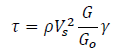
where, τ is the shear stress at the given point, ρ is the mass density of the soil, VS is the shear wave velocity in the given layer, G is the shear modulus at the given point, G0 is the shear modulus at 0% shear strain, γ is the shear strain at the given point.
The maximum value of shear stress for the given layer is then plotted at the depth corresponding to that layer. Using this maximum value, the implied friction angle is then calculated using the following equation:
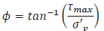
Where 𝜙 is the friction angle, 𝜏𝑚𝑎𝑥 is the maximum shear stress as calculated above, and 𝜎′𝑣 is the effective vertical stress at the mid-depth of each layer.
The user is encouraged to carefully check the provided plots. If the implied strength or friction angle of particular layer is deemed unreasonable, the user should consider modifying the modulus reduction curve for the layer to provide a more realistic implied strength or friction angle.
Water Table
The check box Water Table is used to choose the depth of the water table by clicking the drop-down menu and selecting the layer that the water table will be above.
Bedrock (Halfspace Definition)
As part of the Soil Profile Definition, the user must also define the rock / half-space properties of the bottom of the profile. This can be done by selecting the Bedrock layer.
The user has the option of selecting either an Elastic Half-space or a Rigid Half-space. An elastic half-space should be selected if an outcrop motion is being used and a rigid half-space should be selected if a within motion is being used. If an elastic half-space is being used, the user must supply the shear wave velocity (or modulus), unit weight, and damping ratio of the half-space. If a rigid half-space is being used, no input parameters are required.
In general, the shear wave velocity of the bedrock should be greater than that of the overlying soil profile. It should be noted that the bedrock damping ratio has no effect in time domain analyses and only a negligible effect in frequency domain analyses regardless of the value specified by the user.
If the analysis includes porewater pressure generation and dissipation with a permeable half-space, the user is also given the option to specify the coefficient of consolidation Cv for the halfspace. If no value is specified, RSSeismic will use the coefficient of consolidation Cv of the last layer for the half-space as well. If the user is conducting a frequency domain analysis, deconvolution can be performed rather than a forward analysis.