Response Spectra Calculation Methods
The frequency-domain solution, the Newmark β method and Duhamel integral solutions are the three most common methods employed to estimate the response of Single Degree of Freedom (SDOF) systems and therefore to calculate the response spectra. A brief description is presented for each method to calculate the response of SDOF systems and to solve the dynamic equilibrium equation defined as (Chopra, 1995; Newmark, 1959):
| 𝑚𝑢̈+𝑐𝑢̇+𝑘𝑢=−𝑚𝑢̈𝑔 | Eqn. 1 |
where m, c and k are the mass, the viscous damping and the system stiffness of the SDOF system respectively. 𝑢̈, 𝑢̇ and 𝑢 are the nodal relative accelerations, relative velocities and relative displacements respectively and 𝑢̈𝑔 is the exciting acceleration at the base of the SDOF.
Frequency-domain solution
In the frequency-domain solution, the Fourier Amplitude Spectra (FAS) input motion is modified by a transfer function defined as:
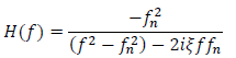 | Eqn. 2 |
where fn is the natural frequency of the oscillator calculated as 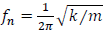 and 𝜉 is the damping ratio calculated as
  . Use of the frequency-domain solution requires FFTs (Fast Fourier Transforms) to move between the frequency-domain, where the oscillator transfer function is applied, and the time-domain, where the peak oscillator response is estimated. Over the frequency range of the ground motion, the frequency-domain solution is exact.
Duhamel integral solution
The second method to compute the response of linear SDOF systems interpolates –commonly assuming linear interpolation– the excitation function (−𝑚𝑢̈𝑔) and solves the equation of motion as the addition of the exact solution for three different parts:
- free-vibration due to initial displacement and velocity conditions
- a response step force (−𝑚𝑢̈𝑔𝑖) with zero initial conditions
- response of the ramp force [−𝑚(𝑢̈𝑔𝑖+1−𝑢̈𝑔𝑖)𝛥𝑡⁄].
The solution in terms of velocities and displacements is presented in the following equations:
| 𝑢̇𝑖+1=𝐴′𝑢𝑖+𝐵′𝑢̇𝑖+𝐶′(−𝑚𝑢̈𝑔𝑖)+𝐷′(−𝑚𝑢̈𝑔𝑖+1) | Eqn. 3 |
| 𝑢𝑖+1=𝐴𝑢𝑖+𝐵𝑢̇𝑖+𝐶(−𝑚𝑢̈𝑔𝑖)+𝐷(−𝑚𝑢̈𝑔𝑖+1) | Eqn. 4 |
where:
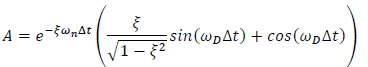 | Eqn. 5 |
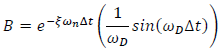 | Eqn. 6 |
 | Eqn. 7 |
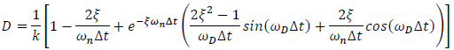 | Eqn. 8 |
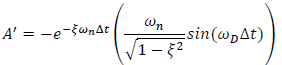 | Eqn. 9 |
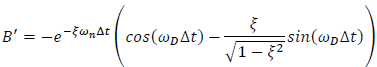 | Eqn. 10 |
 | Eqn. 11 |
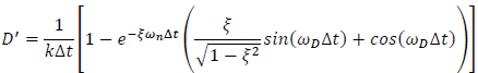 | Eqn. 12 |
Newmark β time integration method in time-domain SDOF analysis
The third method is the Newmark β method. The Newmark β method calculates the nodal relative velocity 𝑢̇𝑖+1and 𝑢𝑖+1 displacements at a time i+1 by using the following equations:
| 𝑢̇𝑖+1=𝑢̇𝑖+[(1−𝛾)Δ𝑡]𝑢̈𝑖+(𝛾Δ𝑡)𝑢̈𝑖+1 | Eqn. 13 |
| 𝑢𝑖+1=𝑢𝑖+(Δ𝑡)𝑢̇𝑖+[(0.5−𝛽)(Δ𝑡)2] 𝑢̈𝑖+[𝛽(Δ𝑡)2]𝑢̈𝑖+1 | Eqn. 14 |
The parameters β and γ define the assumption of the acceleration variation over a time step (Δt) and determine the stability and accuracy of the integration of the method. A unique characteristic of the assumption of average acceleration (β = 0.5 and γ = 0.25) is that the integration is unconditionally stable for any Δt with no numerical damping. For this reason, the Newmark β method with average acceleration is commonly used to model the dynamic response of single and multiple degree of freedom systems.
The Newmark β method has inherent numerical errors associated with the time step of the input motion (Chopra, 1995; Mugan and Hulbe, 2001). These errors generate inaccuracy in the solution resulting in miss-prediction of the high-frequency response. To determine if a motion’s time step is too large to be used directly, the response spectrum calculated with the Newmark β method can be compared with the response spectra calculated by other means, with and without a time step correction in the Motion tab.