Theoretical Overview
Stress strain curves
For concrete, modified Hognestad (1951) is used for the time being. For steel whether rebars, casing or I beam, elastic perfect plastic stress strain is used with yield strength and modulus are input in section design of RSPile reinforced concrete section.
The concrete cylinder strength is given by the user and initial tangent modulus of concrete is taken as Ec=4700(fc’)0.5, fc’ and Ec being in MPa or equivalent equation in imperial units. The ultimate concrete compressive strain is fixed as 0.0038, while strain at maximum stress is taken as 1.7fc’/Ec.
Tension in concrete is considered as long as the stress is less than the modulus of rupture. The used formula for the modulus of rupture is given in ACI 318 code as 0.62(fc’)0.5 MPa.
It is intended to expand the program to include different stress strain curves other than Hognestad curves covering different codes and methods.
Sections of reinforced concrete
The sections considered in RSPile are rectangular and circular sections. They may have a casing, include a single I beam, or having a core in the middle with or without steel liner and concrete filled or not.
Failure conditions
The interaction diagram points are calculated in 5 cases.
Maximum compression in the section which is Pnc = 0.85fc’Ac+ ΣAsfy, with Mn=0.
Maximum tensile force in the section Pnt=As fy with Mn=0
Points where compression controls, i.e. failure in compression of concrete. This happens were the strain at ultimate fiber reaches 0.0038 and steel tensile strain is still below yield.
Points where compression and tension are available in the section. Compression strain reaches 0.0038 but steel tensile strain is allowed to increase.
Points where tension controls the section and concrete is no longer in compression at any point. In this case the strength of the section is calculated at a maximum strain of 0.005.
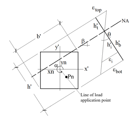
Searching for the neutral axis
The angle of the direction of the point of load application α measured CCW from the x’ axis may be any value between 0 and 360 degrees given by the user. After assigning a value for α the program divides the range of the axial load Pnt to Pnc to a certain number of divisions. For the time being the number of load levels are 20. Then for each load level the program searches for the adequate location of N.A. that will satisfy the equilibrium of the internal action with the external applied axial force with the condition that the direction of load application is in the specified angle. The search ends with a location and orientation of the neutral axis. The angle of the neutral axis β, measured from the x’ axis +ve CCW 0o to 90o and -ve CW 0o to -90o. The neutral axis must lie at an angle in this range -90o to +90o. is varied. After determining β and the location of the neutral axis by its intersection with x’ or y’, the resultant moment of the applied force and the internal forces about the neutral axis is calculated as Mn. The components of Mn, which are Mnx’ and Mny’ will be found based on α.
For a specific axial load chosen by the user the program also calculates all possible points of Mnx’-Mny’ that satisfy equilibrium at failure for α angles from 0o to 360o divided 20 intervals (this will be enhanced in future versions).
Equilibrium is determined based on that the difference in moments and forces are close to zero with certain accuracy. For the time being the accuracy for the axial load equilibrium is 1% which is enough for the construction of the interaction diagram. The minimum error in moments is calculated based on a 1o maximum difference in the angle α (this is to be improved in next versions).
Strains at any level are calculated based on the ultimate strain assumed using the curvature θ which is increase iteratively from 0 to by 0.0001 rad in each step.
Results
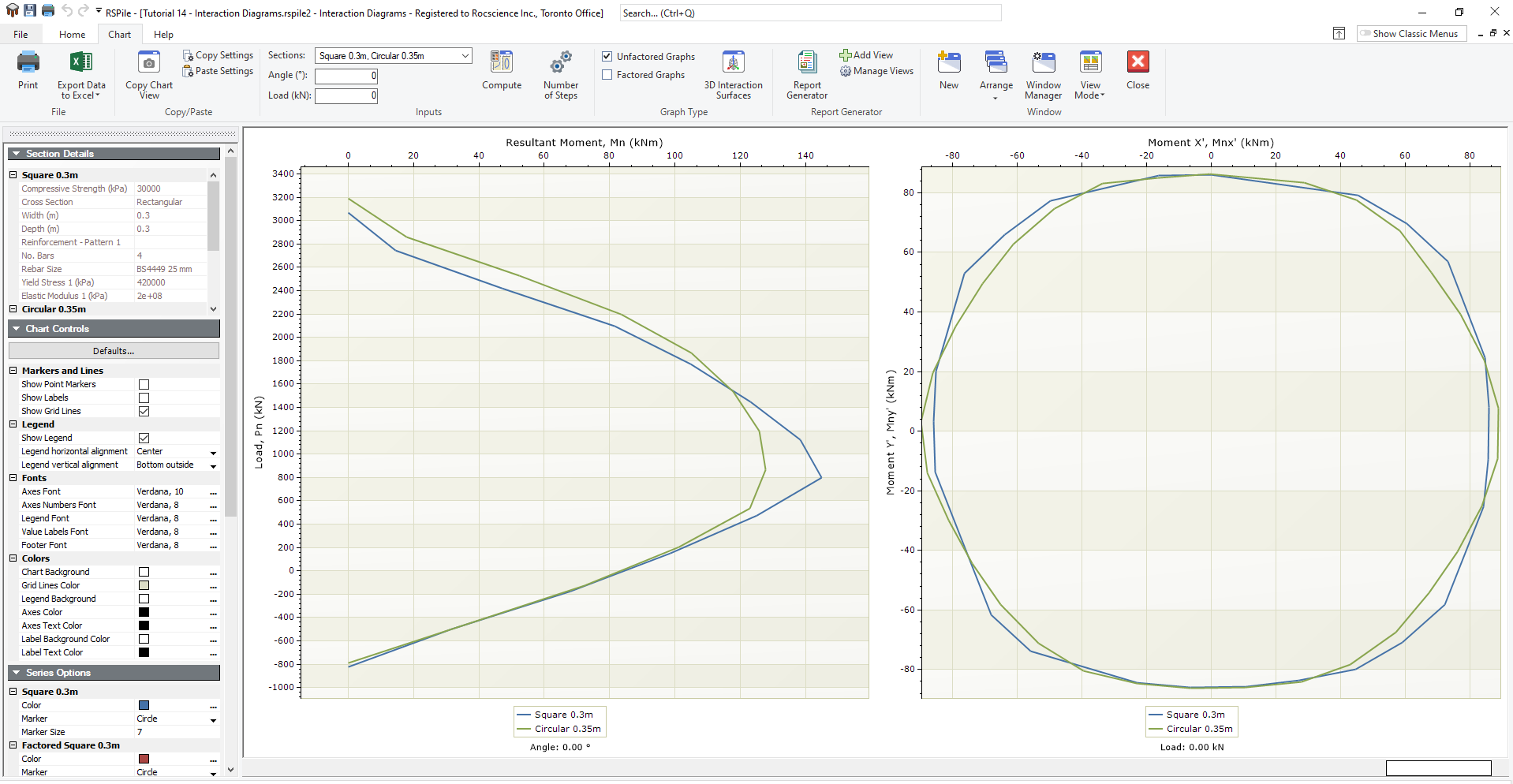
Results are shown if the user chooses graphing the interaction diagram for a section, check tutorial 15. The results are given as Mn-Pn curve for a chosen angle for the direction of point of loading as explained above and a graph for Mnx’-Mny’ for a specific axial load. The load is given +ve for compression in this feature.
Fig.2 shows how RSPile results are presented. The angle for Mn-Pn curve and the load for Mnx’-Mny’ plot, are shown below the graphs.
References
Hognestad, E. (1951): A Study of Combined Bending and Axial Load in Reinforced Concrete Members. University of Illinois Engineering Experiment Station, Bulletin Series No.399, Bulletin No.1, 28pp.
Neville A.M. (1974): Properties of Hardened Concrete. Chapter 3 in “Reinforced Concrete Engineering”, edited by B. Bresler, Vol.1. John Wiley and Sons, New York.
Wang, C. and Salmon, C. G. (1973): Reinforced Concrete Design, 2nd ed., Intext Educational Publishers, New York.