11 - Probabilistic analysis with random shear strength (COV)

1.0 Introduction

This tutorial introduces the ability of Slide2 to define statistical variability in a material's shear strength using the option of a coefficient of variation. This option can be applied to all material strength types, including Shear/Normal, Anisotropic, Discrete functions. The capability to statistically vary strength envelopes (functions) offers an important advantage: it eliminates the need to define variability on multiple individual parameters for a material. This feature is particularly helpful in cases where parameter-specific data may be sparse.

The finished product of this tutorial can be found in the Tutorial 11 COV.slmd data file. All tutorial files installed with Slide2 can be accessed by selecting File > Recent Folders > Tutorials Folder from the Slide2 main menu.

1.1 What is Coefficient of Variation (COV)?

The coefficient of variation is a statistical parameter that measures the relative dispersion (variation) of data around the mean. The COV is defined as the standard deviation divided by the mean and is sometimes shown as a percentage. The higher the COV, the greater the level of variation around the mean.

2.0 Model Geometry

1. Select File > Recent > Tutorials and open Tutorial 11 COV – starting file.

(See Analysis > Project Settings for the parameters set for this tutorial.)

Now let us look at the slope materials and their strength properties, which have been defined already.

2.1 Material properties

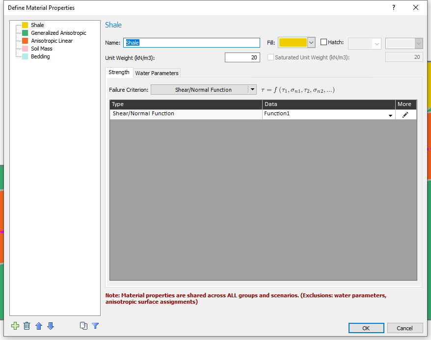
1. Select Properties > Define Materials
   

The slope material consists of five different materials.

• The first material, Shale, has Shear/Normal Function Strength. This strength function allows you to define an arbitrary, non-linear Mohr-Coulomb failure envelope for a material.
Visit the Shear / Normal Strength Function help page to learn how it is defined.

2. Click on the Edit button to see the Shear/Normal function defined for the Shale material. The table of shear/normal values for the function is shown below.



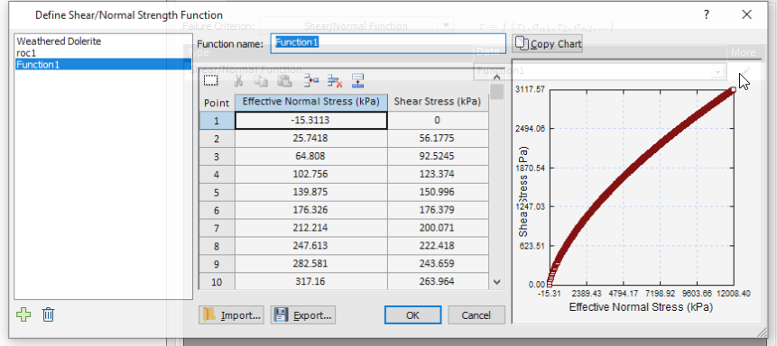
3. Click Cancel to close the dialog and return to the material properties dialog.

• The second material is Generalized Anisotropic. This material has the Generalized Anisotropic Strength type. The Generalized Anisotropic Strength option allows you to create a composite material model made up of two or more of the strength models in Slide2.
To know more about the Generalized Anisotropic Function, see the Generalized Anisotropic help page.

4. Under Strength Parameters, click on the Edit button to view the Generalized Anisotropic Function defined. The function essentially indicates bedding planes (which are weakness planes) that are inclined at -10 to +10 degrees from the horizontal.



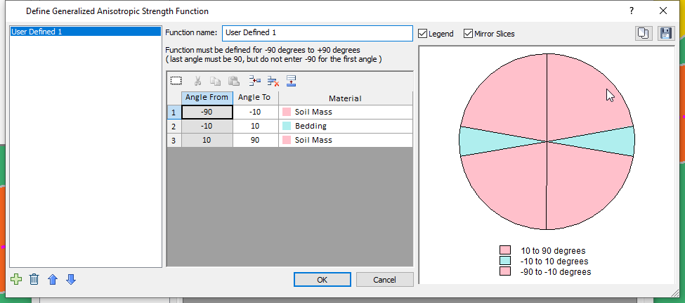
5. Click Cancel to close the dialog when done.

• The third material defined is an Anisotropic Linear material.
See the Anisotropic Linear Strength help page to learn more about the Generalized Anisotropic Function.
• The fourth and fifth materials (Soil Mass and Bedding) have Mohr-Coulomb strength.

6. Click Cancel to close the Define Material Properties dialog. We will run an analysis using the COV option for some of the slope materials.

3.0 COV OPTION

To use COV variability, we must first enable the Probabilistic Analysis option.

1. Select Analysis > Project Settings
2. Click on the Statistics tab and tick the Probabilistic Analysis checkbox.
3. Set the number of samples to 50 (this is done to reduce the computation time while illustrating this type of analysis)
4. Set the Sampling Method to Latin Hypercube and the Analysis Type to Overall Slope.
   
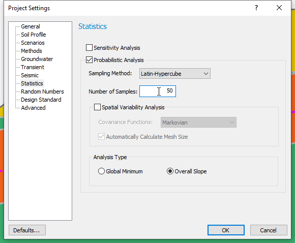
5. Click OK to close the Project Settings dialog.
   
   Now the Statistics menu will appear in the menu bar.
   
   
6. Select Statistics > Materials to open the Material Statistics dialog.
   
   In this dialog we will define shear strength using COV for the Shale, Generalized Anisotropic and Anisotropic Linear materials.
   
   
7. Check the Define shear strength using COV box. We will specify a lognormal statistical distribution for the Shale material and a coefficient of variation of 0.1, as shown in the dialog below.
   
   
   This means that the shear strength of the Shale will vary according to the lognormal distribution, with a coefficient of variation of 0.1. This option essentially specifies the standard deviation at any location along the shear/normal function as 10% of the mean value (defined by the strength curve).

Select the COV table button on the Material Statistics dialog (outlined in red on the image above) to see the typical range of values for different materials.

8. Now click on Generalized Anisotropic in the sidebar and check the Define shear strength using COV box.
   
9. We will use a Uniform statistical distribution.
   Notice that the Minimum and Maximum fields now replace the COV box. The uniform, triangular, and exponential distributions do not use standard deviation as a parameter.
   
10. Enter a Minimum value of 0.75 and a Maximum value of 1.25.
    
    
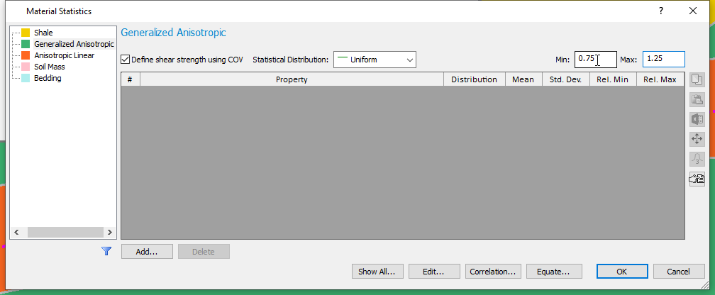
    For each simulation, the shear strength values calculated at location will vary uniformly between a lower and upper range defined as the shear strength values multiplied by 0.75 and 1.25, respectively.
    
11. Select the Anisotropic Linear material.
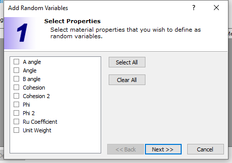
12. Click the Add button. Notice that by using COV, we eliminate the need to define variability for all these individual parameters associated with Anisotropic Linear. Click Cancel.
    
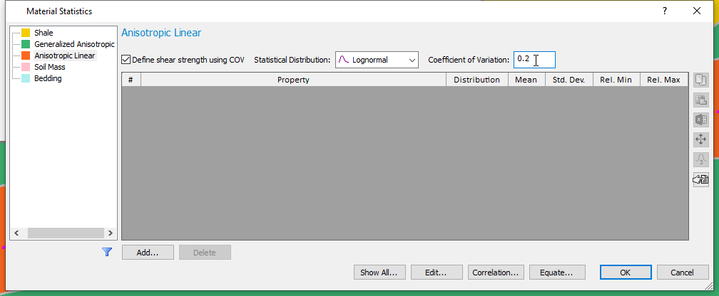
13. Now, define a COV random variable with Lognormal Distribution and a Coefficient of Variation of 0.2, as shown in the dialog below.
    
    
    
    
Notice that you can also define random shear for Soil Mass and Bedding materials, which make up the Generalized Anisotropic material. Keep in mind that if you do so, these random variables will be independent of the random shear in Generalized Anisotropic, meaning they will not be derived from the Generalized Anisotropic material’s random shear. However, if you would like them to be dependent, you can always define correlation using the Correlation button as you see fit.

14. Click OK.

We will now run a non-circular, particle swarm search analysis. (See Surfaces > Surface Options)

4.0 Computation and Interpretation

1. Select Analysis > Compute and run the COV analysis. The computation may take a few minutes.
2. Select Analysis > Interpret to view results after computations are done.

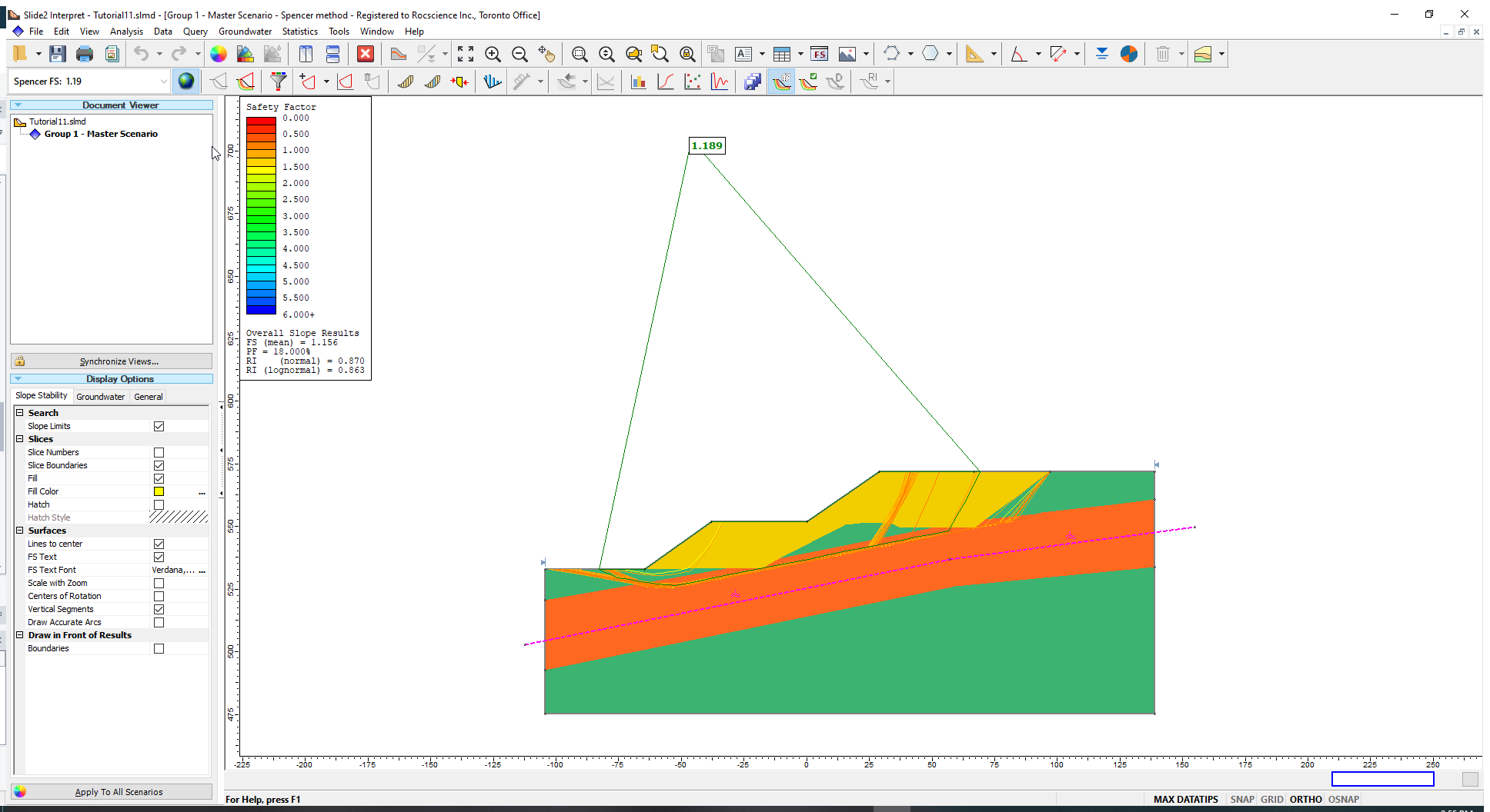
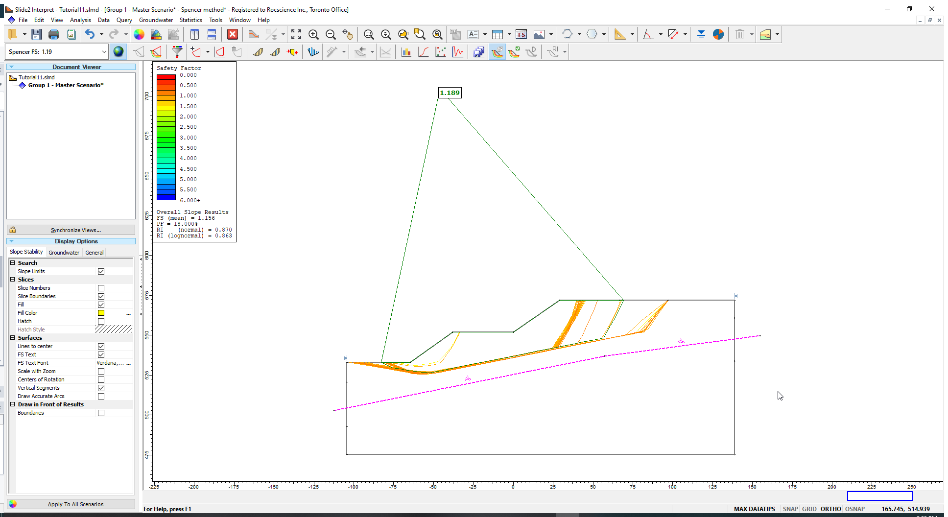
The Probability of Failure for the COV analysis is 18%. Notice that the failure surfaces mostly conform to (have significant sections parallel to and passing through) the anisotropic surface that defines the Anisotropic Linear material.

To see the minimum surfaces determined for each of the statistical simulations properly:

1. Go to the Display Options in the left-hand sidebar (or access them from View > Display Options).
2. In the General tab, turn off the Material Colors.
   
   Now let us plot the Shale Shear Strength Factor.
   
3. Select Statistics > Histogram Plot and plot the Shale Shear Strength Factor.
   
   

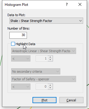
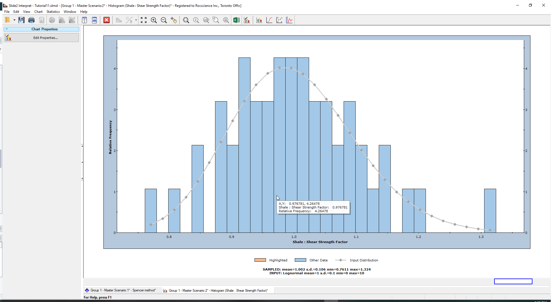
You will see the histogram below along with the originally specified lognormal distribution for the Shale Shear Strength Factors. These factors are generated from a lognormal distribution with a mean value of 1. The originally specified Shear/Normal Strength Function is then multiplied by these factors to obtain the lognormal distributed strength variation.

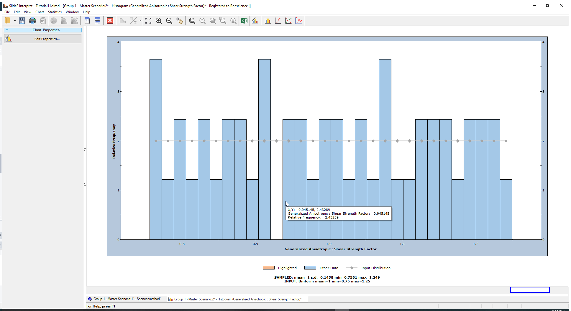
Let us plot the Generalized Anisotropic Shear Strength Factor.

1. Right-click on the plot and select Change Plot Data
   
2. From the ensuing pop-up dialog, select the Generalized Anisotropic Shear Strength Factor and plot the histogram.

You will now see a uniformly distributed histogram ranging from approximately 0.75 to 1.25. This is in line with the range specified in the material statistics dialog.

You may also switch the plot data to Factor of Safety to view its histogram. You can right-click on the chart again and select Best Fit Distribution from the pop-up.

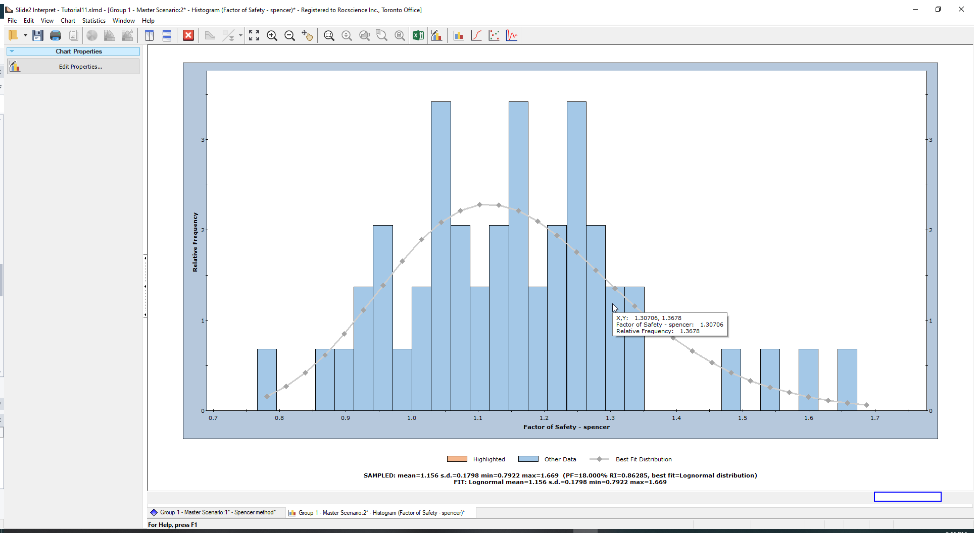
These are the 50 factor of safety values computed from the analysis.

5.0 Additional Exercise

For the sake of speed, we computed only a small number of simulations (50) and therefore saw a small number of surfaces in varying locations based on the varying shear strength. As an additional exercise, you can run 1000 simulations and analyze the resulting failure modes and statistical results.

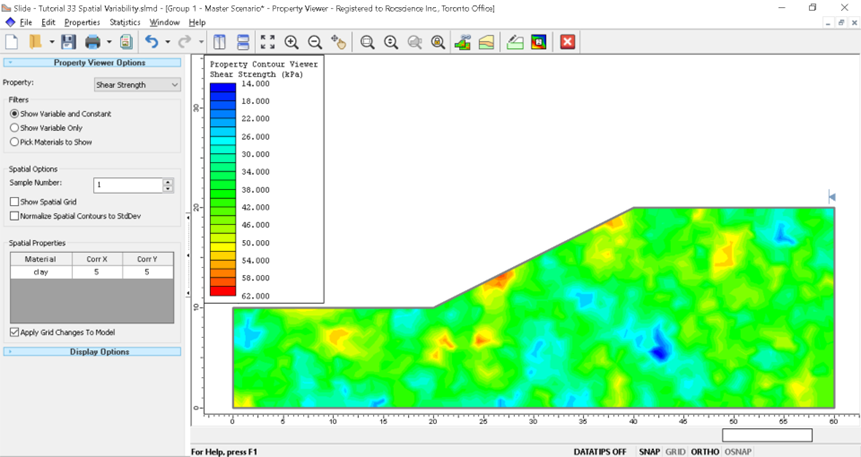
The COV option is also available for spatially variable strength types. Try out Tutorial 10 - Spatial Variability with random shear strength and compare the results to those obtained when we assume random cohesion and friction angle statistical variations.

This concludes the COV tutorial.