3 - Water Pressure Grid Tutorial

1.0 Introduction

Pore water pressures significantly influence the stability of slopes and must be considered when analyzing stability. There are different methods of modelling pore water pressure in Slide2.

This tutorial will perform a stability analysis of an embankment dam with pore water pressure conditions defined using pore pressure values at discrete points (Water Pressure Grid) within the dam and foundation.

The Water Pressure Grid option may comprise groundwater pore pressure distributions defined as Total Head, Pressure Head or Pore Pressure values.

We will use Water Pressure Grid (Total head) for our current tutorial. The pressure at each grid point is defined by X and Y coordinates and a value (in this tutorial, Total Head)

A water pressure grid of total head values has already been generated and will be imported for this tutorial.

At the end of this tutorial, you will have learned how to:

• Import a pore pressure grid from hydrogeological software or field records (saved in PWP file format) into a slope
• Visualize slope pore pressure contours
• Graph pore pressures along the critical slip surface

You can find a finished version of this tutorial in the Tutorial 03 Water Pressure Grid.slmd data file by selecting File> Recent > Tutorials folder from the Slide2 main menu.

2.0 Geometry of Model

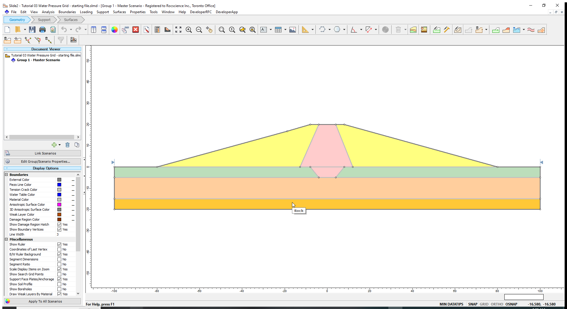
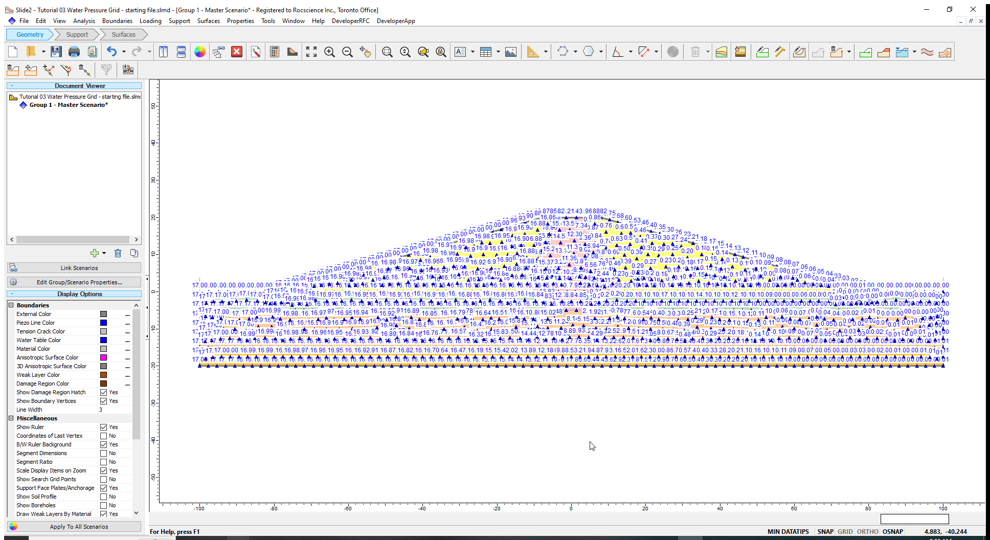
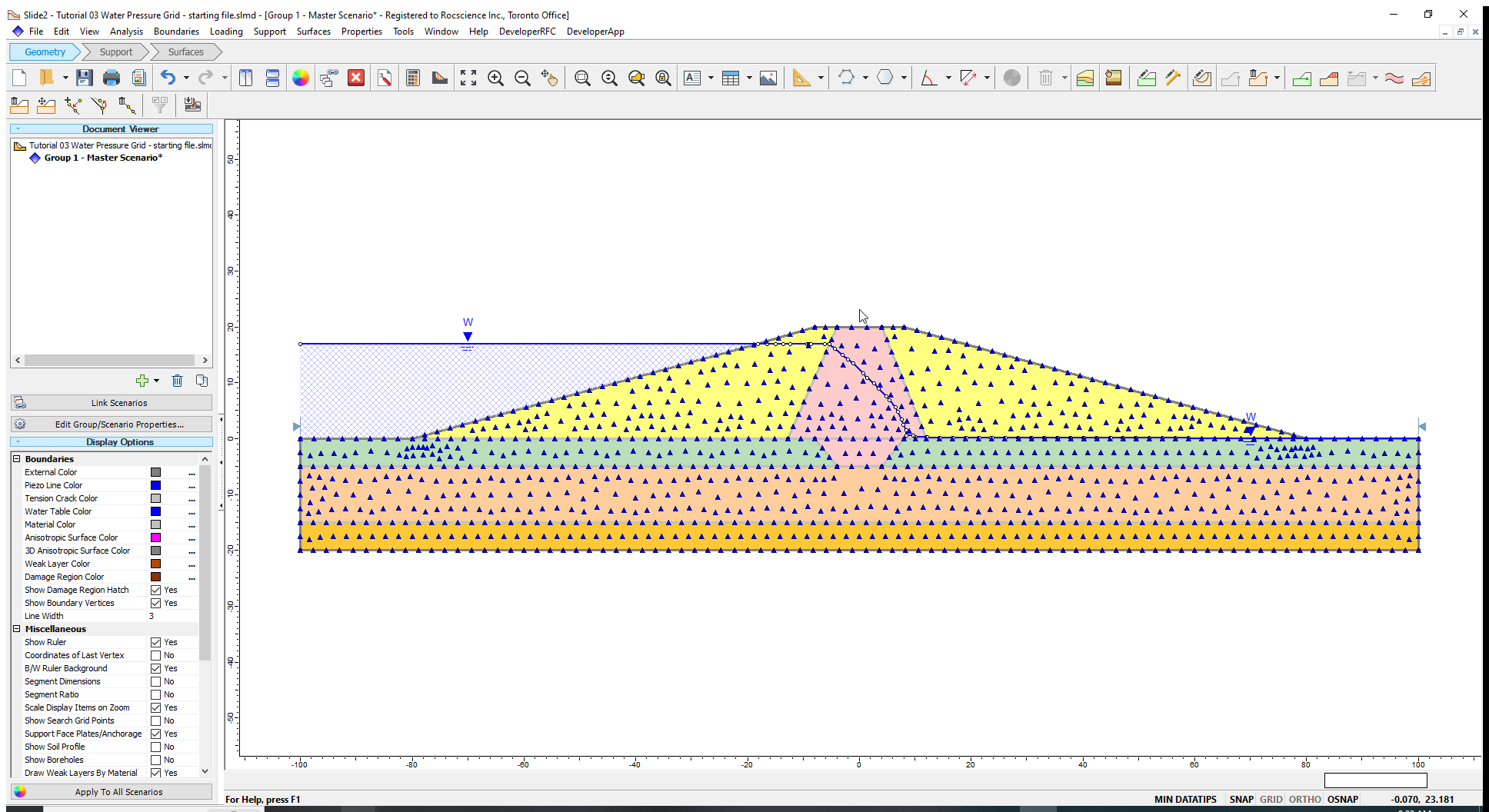
We will use an embankment dam (consisting of two shell zones and a core) founded on the multi-layered (stratified) ground. The material properties are already defined in a starting file, which we will open.

1. Click the drop down arrow to the right of the Openicon and select the Tutorials Folder.
2. Select Tutorial 03 Water Pressure Grid – starting file.slmd and click Open to open the starting model.

The model is shown below.



3. Select Analysis > Project Settings

You will see that Bishop Simplified, Spencer and GLE Morgenstern-Price are the Methods of Analysis set for the tutorial and 'Right to Left’ is the failure direction.

2.1 PORE PRESSURE CALCULATION AND VISUALIZATION

We will use the water pressure grid to specify pore pressures in the embankment and foundation. To do so, we will first select the Grid (Total Head) as the Method. We will then import a water pressure grid file.

1. In Project Settings, select the Groundwater tab.
2. Under Groundwater methods select Grid (Total Head).



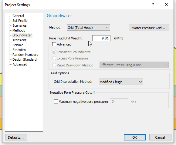
3. Click Water Pressure Grid to open a water pressure grid dialog.



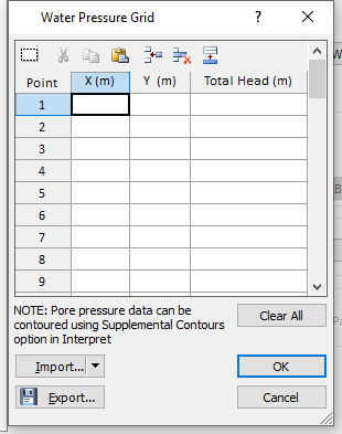
4. Click the Import button to open the Tutorial 03 folder.
5. Navigate to the tutorials folder and locate Tutorial 03 Water Pressure Grid (Total Head).pwp. Select the file and click Open. The water pressure grid values will be imported into the table as X and Y coordinates and a Total head value for each point.
6. The water pressure grid values will be imported into the table as X and Y coordinates and a Total head value for each point. Slide2 offers several different methods for interpolating pore pressure values in-between grid points. We will use the default method (Local Thin-Plate Spline). See the Interpolation Methods help page for a description of the various Grid Interpolation Methods.
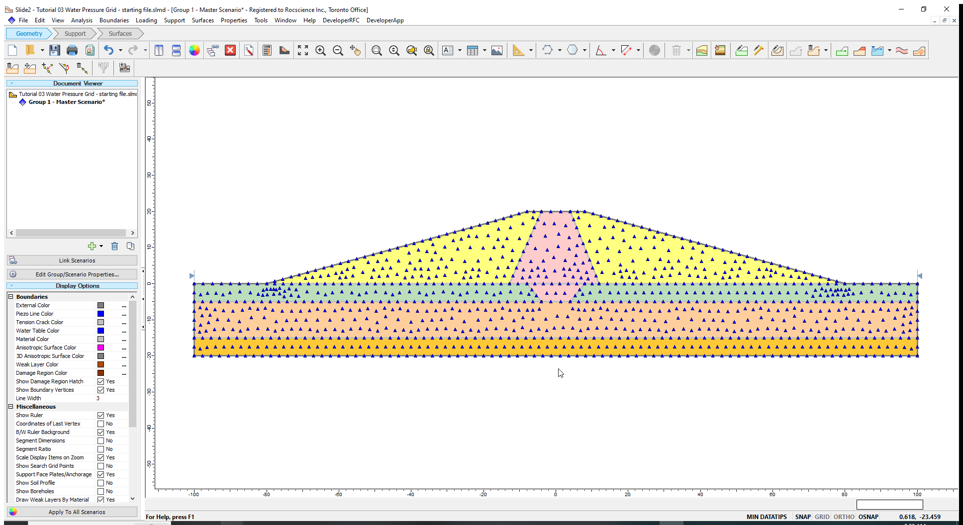
7. Click OK to close the Project Settings dialog. The grid locations will be displayed on the model.

2.2 PORE PRESSURE VISUALIZATION

To display the imported grid values on your model:

1. Right-click on the model.
2. Select Display Options
3. Check the Water Pressure Grid Values box on the dialog.
4. The Total Head values will be displayed on the model. Click Done.

Follow the same steps to turn off the grid values.

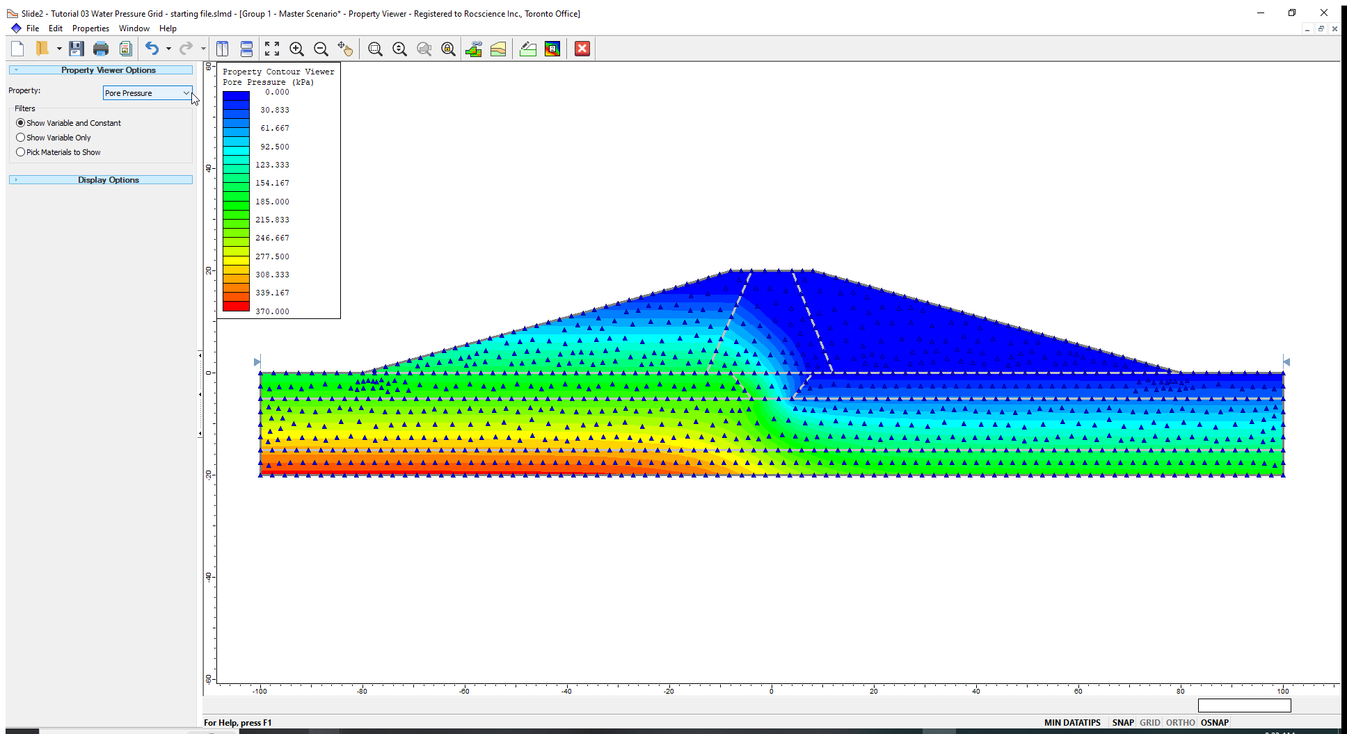
In Slide2, you can visualize the contours of material properties in the Property Viewer, which helps users better appreciate the spatial distributions of these properties. We will visualize the pore pressure contours of our model.

• Select Analysis > Property Viewer

Pore pressures contours are displayed. (Using the Property field under the Property Viewer Options on the left side of the program interface.)

• Click on the Close to close the Property Viewer.

2.3 WATER TABLE

In Slide2, ponded water loads on surfaces are only applied if a water table is specified or finite element seepage analysis is conducted. Pore pressure grids (and piezometric lines) DO NOT apply the weight of ponded water. In the current tutorial, we will define ponded water loading by applying a water table, which will be imported.

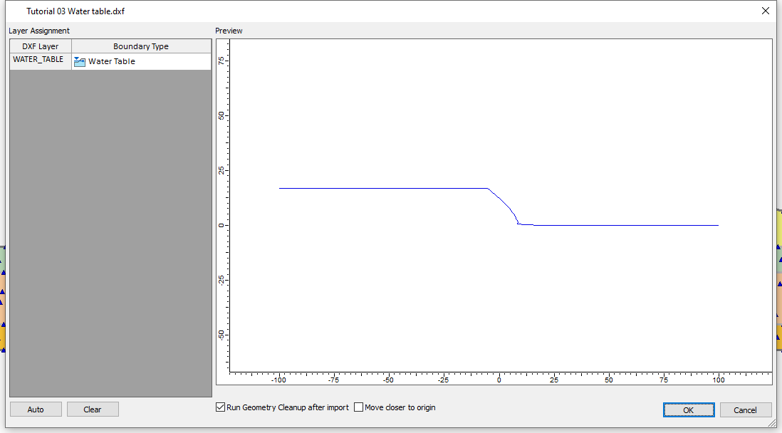
1. Go to File > Import> Import DXF and navigate to the tutorials folder.
2. Select the file Tutorial 03 Water table.dxf and click Open.
3. Ensure the Boundary Type is set to Water Table and click OK.



4. Assign the water table to all the materials and click OK.

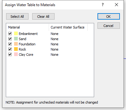
The water table and ponded water loading will now be added to our model.

3.0 Overall Slope Stability Analysis

We will analyze the overall stability of the upstream face of the dam. In order to obtain the overall slip surface for this example, we will have to define two sets of slope limits. (Using only one set of limits results in the identification of localized failure near the upstream crest.)

1. Select Surfaces > Slope Limits > Define Limits
2. Enter the first and second set of limits in the dialog and click OK.

Left x-coordinate	-100
Right x-coordinate	-69.3
Second set of limits
Left x-coordinate	-38.7
Right x-coordinate	-8

4.0 Computing and Interpreting Results

We will now determine the Global minimum surface of the embankment’s upstream side embankment using the non-circular slip surface option and the Cuckoo-search method.

1. Select Analysis > Compute or click on the Compute icon in the toolbar.



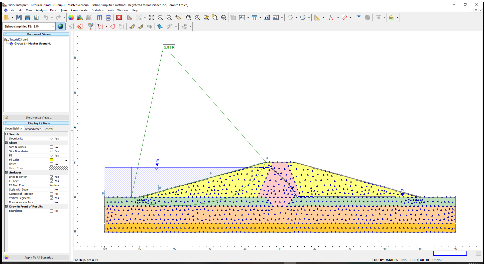
2. Select Analysis > Interpret or click on the Interpret icon in the toolbar.

The critical slip surface for the Bishop Simplified Method and its corresponding Factor of safety is displayed in Interpret. You can view the results for the other methods from the Factor of Safety display box.

We can graph the pore pressures along critical slip surfaces and will do so for the Bishop Simplified method.

To do this:

1. Right-click on the global minimum surface and select Add Query
2. In the Multiple Surfaces dialog click OK. The slip surface will change from green to black if it is successfully queried.
3. Select Query > Graph Query The Graph Slice Data dialog will open.



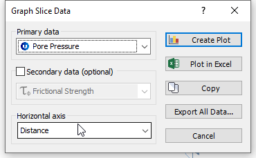
4. Since we are plotting the pore pressures, we will select the following parameters:

Primary data: Pore Pressure

Horizontal axis: Distance

5. Click Create Plot.

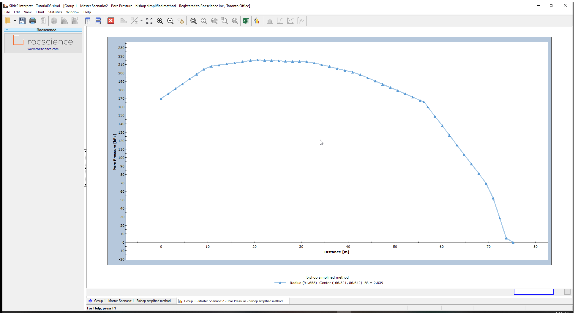
The pore pressure graph is shown above.