22 - Weak Layers

1.0 Introduction

This tutorial will analyze two slopes. The first slope is a simple example which will consider weak layers using two different approaches. The second slope is a more complex example that will explore the Weak Layer Handling algorithms.

First, what do we mean by weak layer? There are TWO ways to consider a weak layer in Slide2:

Method 1: Weak layer as thin material region

In typical slope stability modelling, a weak layer is defined as a thin material layer (using material boundaries) bounded by two stronger material zones. The layer has a finite thickness and is assigned material properties. This method of modelling weak layers is commonly used and works very well in most circumstances. The advanced search algorithms in Slide2 can locate critical slip surfaces even in thin irregular weak layers, with excellent results in most cases.

However, there are some limitations to this method:

• For very thin weak layers (thickness approaching zero), or highly irregular non-linear weak layers, even the best search algorithms can have trouble locating slip surfaces within such layers. In some cases, the user may be forced to define a search polyline inside a finite weak layer, to focus the search within the weak layer.
• If a weak layer represents an interface (with zero thickness), then the user is forced to create a thin material layer with a finite thickness to model the interface since you cannot create a zero-thickness material. Modelling a geomembrane interface in a landfill is such an example.

Method 2: Weak Layer Boundary

Due to the above-described limitations, Slide2 offers a second method for modelling weak layers that use the Weak Layer Boundary option. This approach defines a weak layer using a polyline that is assigned material (strength) properties.

The advantage of using the Weak Layer polyline, is that the search algorithms will attempt to “follow” the weak layer polyline, to generate slip surfaces along the polyline (in this sense, a weak layer polyline behaves as a search focus object). We are forcing the search algorithm to see the weak region.

2.0 Example 1: Simple Weak Layer Model with Two Approaches

2.1 Model Geometry

1. Select File > Recent Folders > Tutorials Folder and open the file Tutorial 22 Weak Layer Ex1 – starting file. Slmd
2. Double-click on the green material to see the properties of the weak layer (or select Properties > Define Materials and select the Weak Layer material from the list).

Notice that it has a cohesion of 0 and is significantly weaker than the Soil material. This group constitutes Method 1 – the analysis of the weak layer as a regular material region.



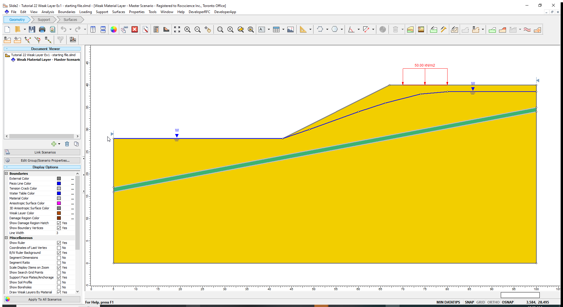
Now we will create a group for Method 2, where we will assign the weak layer boundary to the middle of the physical weak layer in the image above.

3. In the Document Viewer, right-click on Weak Material Layer and select Duplicate Group.
4. Rename Group 2 to Weak Layer Boundary.
5. Select Boundaries > Add Weak Layer in the menu.
6. Enter the vertices of the boundary, (5, 16.5) and (100, 34.5), in the activated Prompt line. (Press Enter once after entering the first vertex and twice after entering the second vertex.)
7. A Weak Layer 1 Property dialog will appear. Select the weak layer material from the drop-down list as shown in the image below. This indicates that the polyline will have the properties of this material.
   
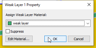
8. Click OK to close the dialog.
The Suppress checkbox can be toggled to exclude the weak layer from the analysis without needing to delete it. They can be unsuppressed by right-clicking the weak layer and unchecking the Suppress option.

The weak layer has been defined.

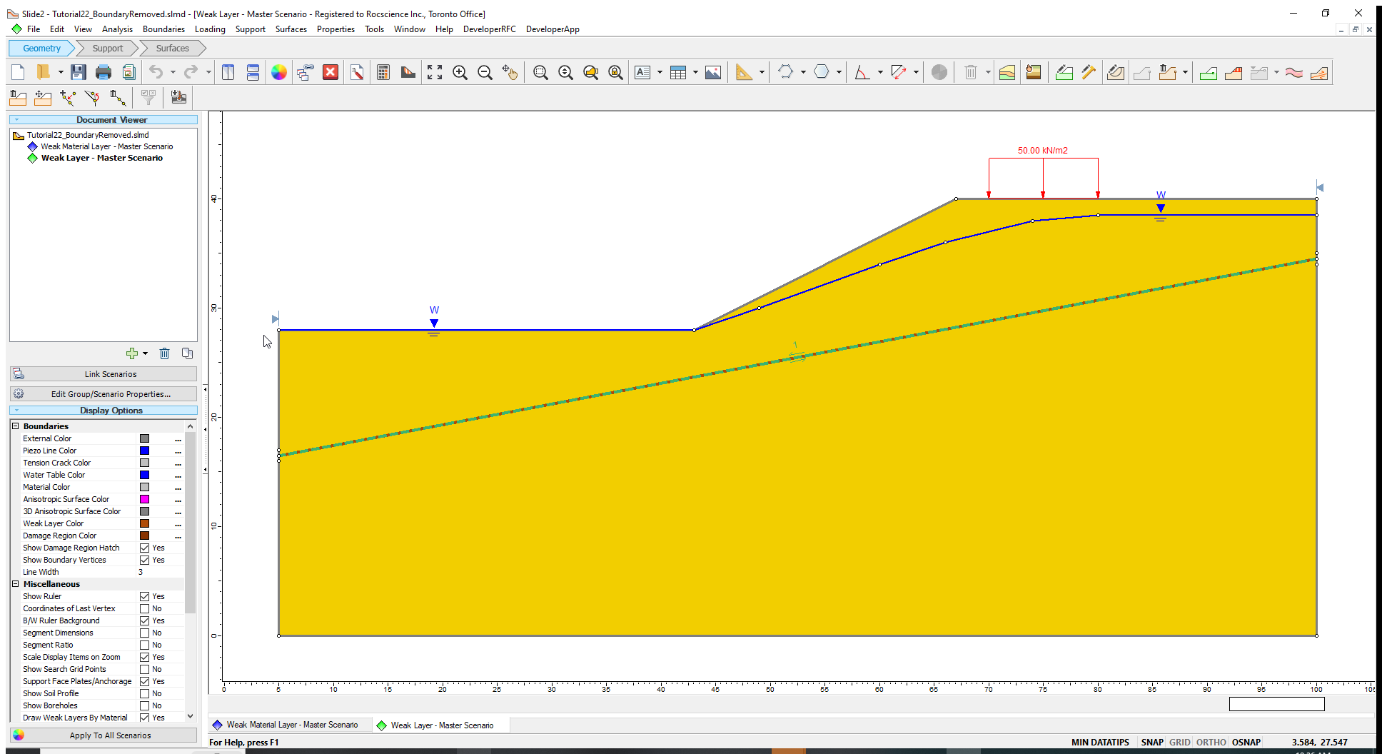
We can now remove the weak material zone.

9. Right-click on the material boundaries (grey) of the green layer and select Delete Boundary. You will have to do this twice.

Your model should look as shown below.

Now we will compute both Groups and interpret the results.

2.2 Computation and Interpretation

1. Run the analysis for both groups (Analysis > Compute ) and interpret the results (Analysis > Interpret ).
2. Select Window > Tile Vertically .

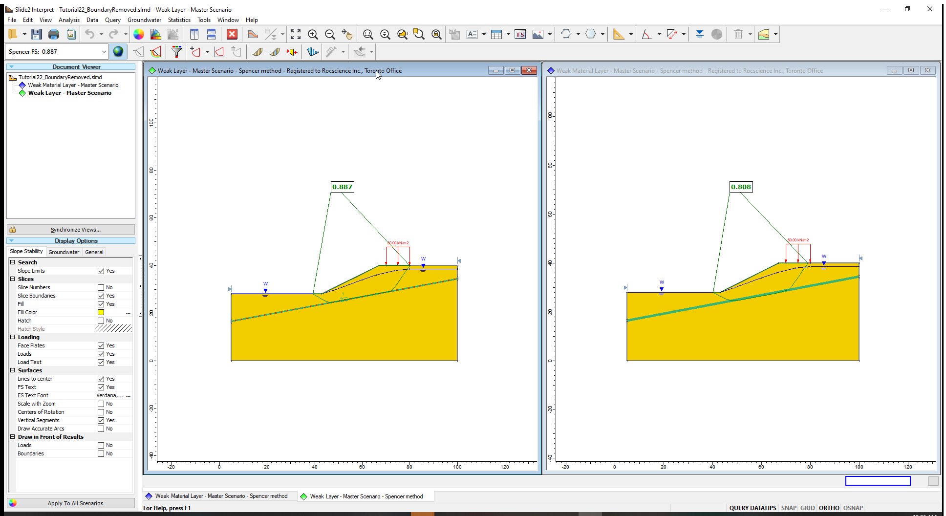
The failure surfaces are very similar, both conforming to the thin weak layer. The results are slightly different because the critical failure surface in the Weak Material Layer group passes through more of the weak layer material (since it has a thickness of 1 metre), slightly lowering the FS.

Now let us look at a more complex model.

3.0 Example 2: Complex Weak Layer Model

In some cases, there may be multiple weak layers that overlap in the model. Sometimes, the material beneath a weak layer can be weaker than the weak layer itself. When the Weak Layer Handling feature is set to Automatic Case Generation or Heuristic (when the search method is Particle Swarm), Slide2 can determine which configuration of weak layers produces the most critical slip surfaces. This is explored below:

1. Go to File > Recent > Tutorials and open the file Tutorial 22 Weak Layer Ex2. slmd.



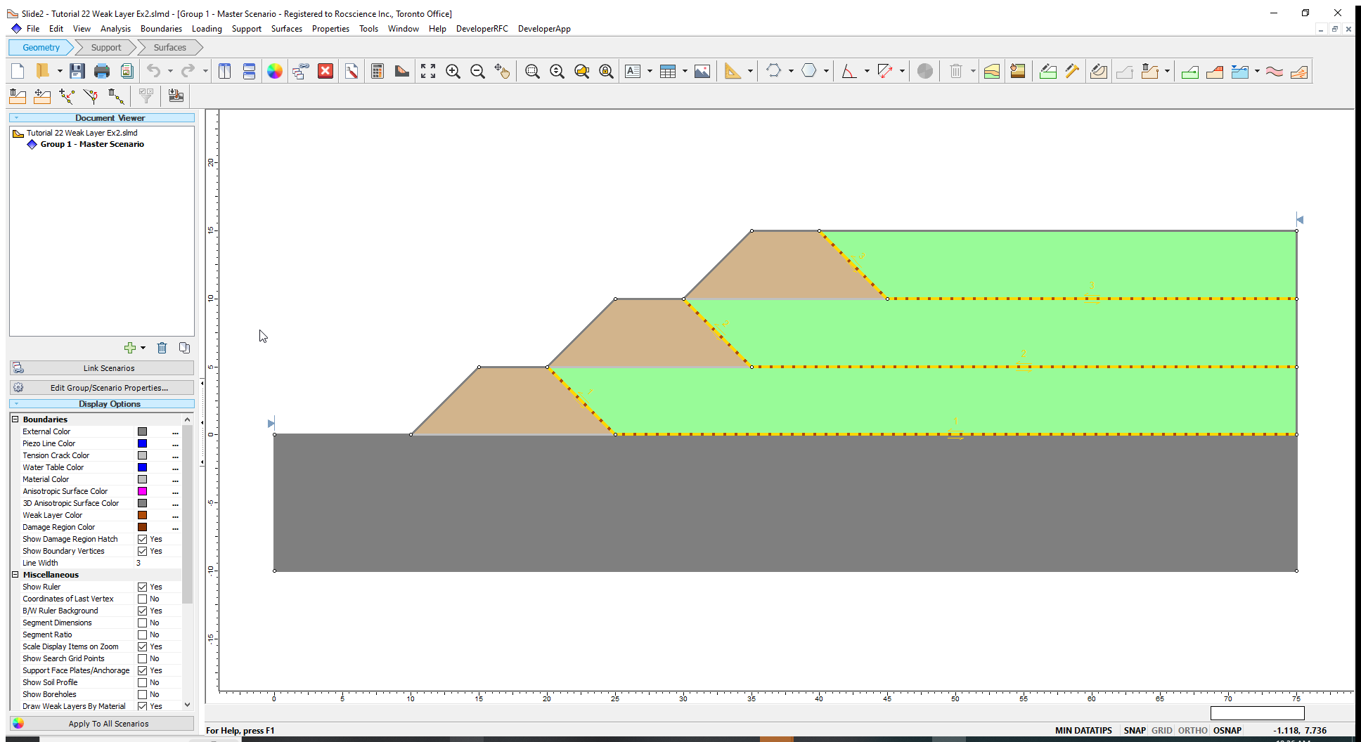
2. Hover the cursor over the different materials and notice that the green material is waste, the brown material is a berm, and the grey material is the native soil underlying the landfill.
If you don’t see any hover over text, click the DATATIPS button in the bottom right of the screen to turn them on.

Notice that three weak layer boundaries have been defined in yellow – if you hover over these you will see that the material is called “Lining” – these represent liners that are containing the green waste material. Since lining is of almost no thickness, a weak layer boundary is the best option for modeling.

Now, we must indicate how the weak layers should be handled in the analysis.

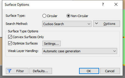
3. Select Surfaces > Surface Options .
4. We will use the default Weak Layer Handling option: Automatic case generation. This option automatically checks which layer(s) will generate the minimum factor of safety for a given slip surface by activating and deactivating the various weak layers intersected by the slip surface until the best combination is found.



The “Always snap to highest layer” option will only consider the top weak layer. This is appropriate in the case of a single weak layer, or in the case of multiple weak layers side by side, in which case you will save computation time by using this option.
If there are many weak layers in the model, “Automatic case generation” may perform slowly. The more efficient Heuristic method is available if you change the search method to Particle Swarm Search.
5. Click OK to close the dialog.
6. Run the analysis (select Analysis > Compute ) and interpret the results (select Analysis > Interpret ).

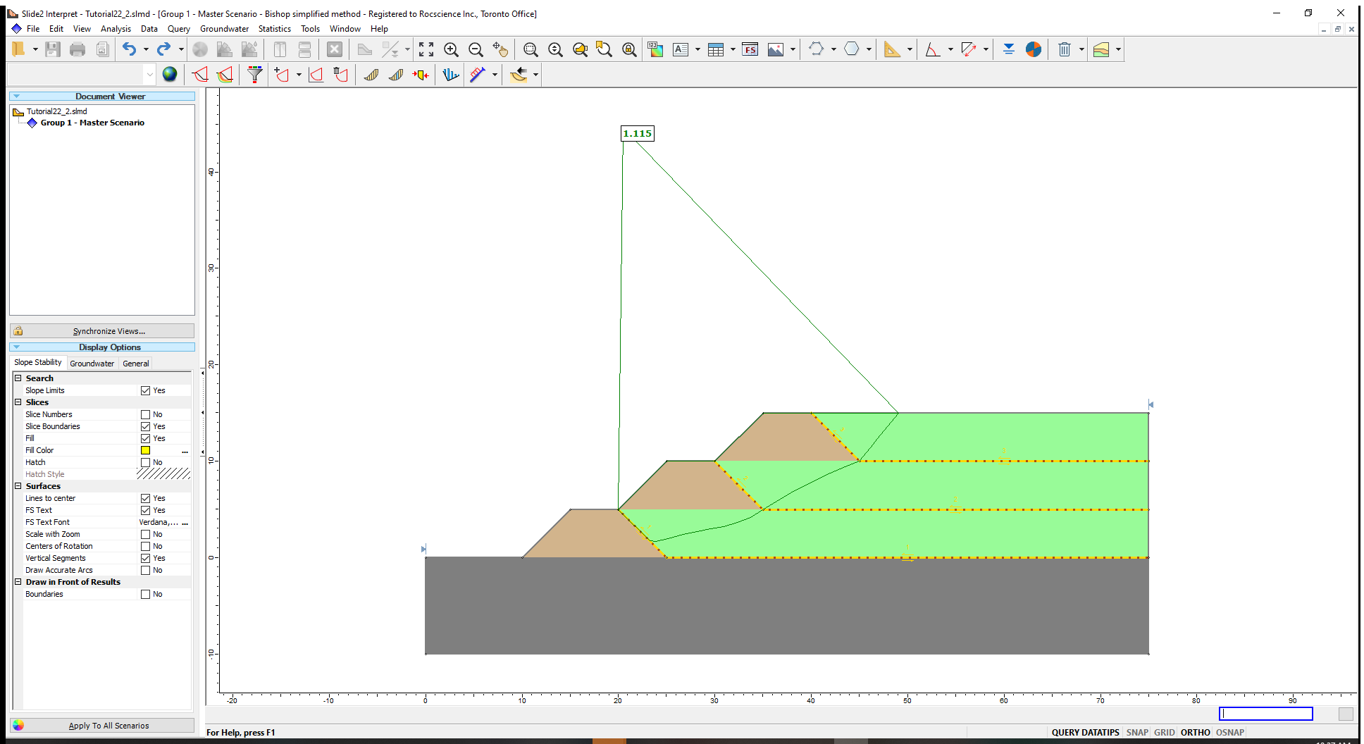
Notice that the critical mechanism does not travel along the top two liners (weak layers); it only travels along a portion (along the berm face) of the bottom liner. This means that the best combination found by the Weak Layer Handling algorithm was to turn the top two weak layers off and the bottom one on.

3.1 Additional Exercise

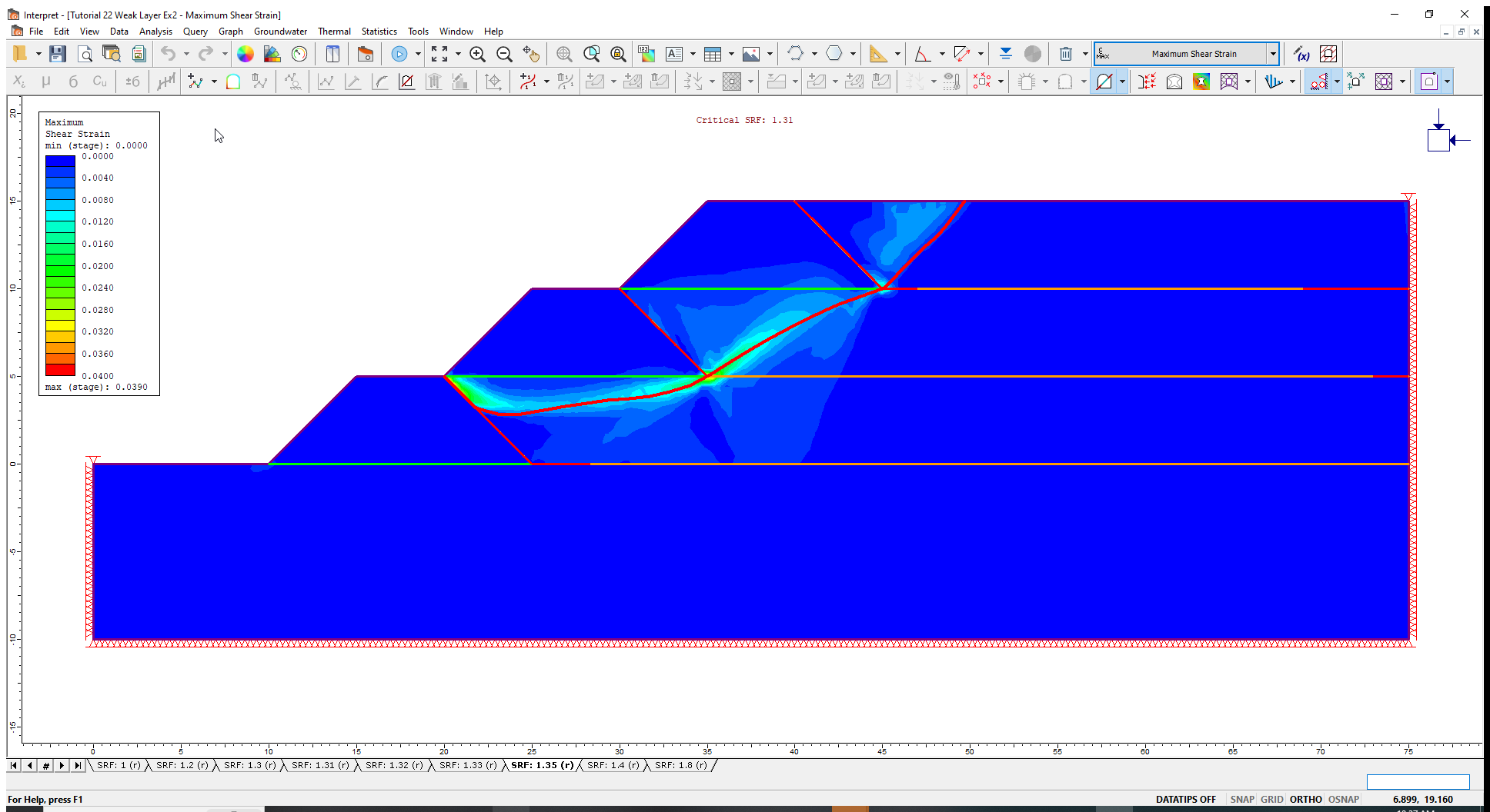
The Global Minimum result can be cross-referenced with RS2 using shear strength reduction.

The maximum shear strain results are shown below (blue = no strain, and lighter colours representing increasing strain). The areas of maximum strain in the model match the critical slip surface obtained in Slide2 (shown in red). As well, RS2 reports a critical strength reduction factor that is similar to the factor of safety in Slide2.

4.0 Limitations

Please see Weak Layer Overview for a detailed discussion of the limitations of the weak layer feature in Slide2. These limitations concern models that have discontinuous and/or vertical weak layers.

This concludes the Weak Layer tutorial.