25 - Seismic Analysis with Newmark Method

1.0 Introduction

This tutorial will demonstrate three ways of modeling the impact of seismic loads on slope stability in Slide2.

At the end of this tutorial, we will know how to do the following:

• Apply pseudostatic seismic loading
• Determine critical seismic coefficient (Ky)
• Run a Newmark displacement analysis

Finished Product

The finished product of this tutorial can be found in Tutorial 25 Seismic Analysis.slmd data file. All tutorial files installed with Slide2 can be accessed by selecting File > Recent Folders > Tutorials Folder from the Slide2 main menu.

2.0 Model Geometry

1. Select File > Recent Folders > Tutorials Folder.
2. Open the file Tutorial 25 Seismic Analysis - starting file.slmd.

The model is based on the non-homogeneous, three-layer slope in Slide2 Verification Problem #4.

The file has an initial scenario labelled, ‘No Seismic’. We will first run this analysis to determine the factor of safety of the slope when no seismic loads are considered.

3. Run the analysis (Analysis > Compute ) and interpret results (Analysis > Interpret ) when computations are done.

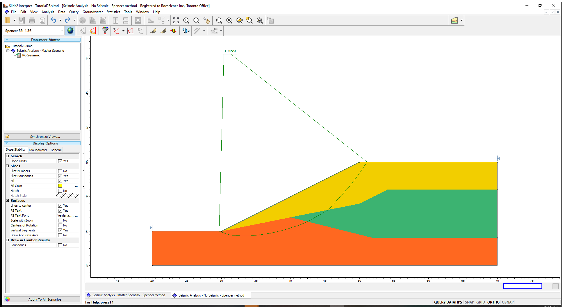
The Spencer factor of safety for this scenario does not consider any seismic effects.

4. Return to the Slide2 Model program.

3.0 Pseudostatic Seismic Loading

1. In the Document Viewer, right-click on No Seismic and select Duplicate Scenario.
2. Right-click on this new scenario and select Rename.
3. Enter Seismic = 0.15 as the scenario name.
   
4. Click Save and Close.

Now we will introduce a pseudo-static seismic load by specifying a horizontal seismic load coefficient, which is used to determine the seismic force applied to the slope.

In Slide2, pseudo-static seismic loads can be applied in the horizontal and vertical directions. In this tutorial, seismic loads will only be applied in the horizontal direction.

5. Select Loading > Seismic Load to open the Seismic Load dialog.
6. In the dialog, enter a Horizontal = 0.15 positive in the direction of failure.
   
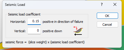
7. Click OK to close the dialog.

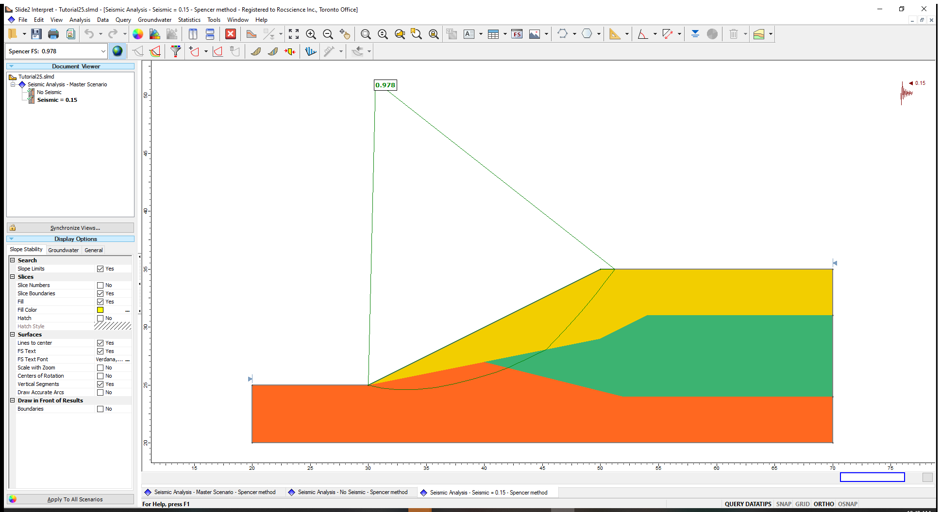
Notice that a seismic loading icon is now added to the top right side of the model.

8. Run the analysis (Analysis > Compute ) and interpret the results (Analysis > Interpret ) when computations are done.

3.1 Computation and Interpretation

With the addition of horizontal seismic loading, the Global Minimum safety factor drops significantly, indicating that the seismic load destabilizes the slope.

1. Return to the Slide2 Model program.

4.0 Critical Seismic Coefficient (Ky) Analysis

Now let us determine the critical (minimum) seismic coefficient (Ky) that brings the slope to the verge of instability i.e., results in FS = 1. This is done using the advanced seismic analysis option in Slide2.

1. In the Document Viewer, duplicate the Seismic = 0.15 scenario and rename the new scenario Critical Acceleration.

To run the advanced seismic analysis:

2. Open the Project Settings dialog (Analysis > Project Settings ).
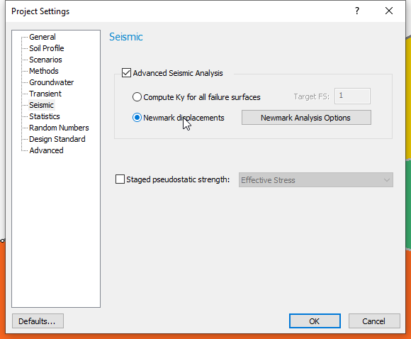
3. Select the Seismic tab and tick the Advanced Seismic Analysis checkbox.
4. The “Compute Ky for all failure surfaces” radio option is selected, and the Target FS is 1. This option will compute Ky for all failure surfaces.
   
5. Click OK to close the dialog.
6. Compute the scenario (Analysis > Compute ) and interpret the results (Analysis > Interpret ) once the computations are done.

4.1 Computation and Interpretation

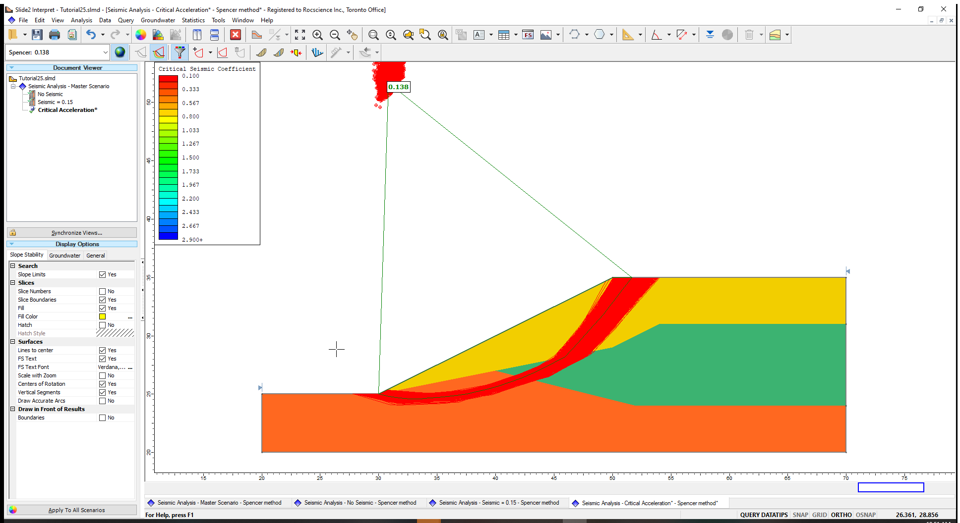
As shown below, you should see a critical slip surface with the associated critical seismic coefficient, Ky. Note that it is lower than the Ky of 0.15 we defined in the previous scenario.

1. To view all surfaces, simply click on the All Surfaces icon.

These failure surfaces are assigned different colours (described on the displayed legend) that correspond to their associated critical seismic coefficients.

Next, let us filter out all surfaces with a critical seismic coefficient (Ky) below 0.15 (the seismic coefficient specified earlier).

2. Go to Data > Filter Surfaces
3. In the Filter Surfaces dialog, select the Surfaces with a Ky below option and enter a value of 0.15.
   
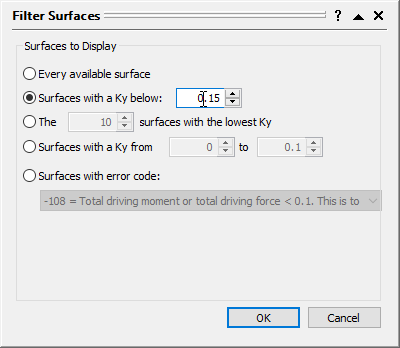
4. Click OK.

There are a number of unstable surfaces for this model, wherein a seismic coefficient less than 0.15 would result in a destabilized slope. This makes sense, since the Global Minimum factor of safety for the Seismic = 0.15 scenario, is below one.

5. Return to the Modeler.

5.0 Newmark Displacement Analysis

The Newmark analysis in Slide2 is based on the program SLAMMER, developed by the U.S. Geological Survey. We gratefully acknowledge the permission to use the SLAMMER code in Slide2 granted by Dr. Jibson and Dr. Rathje.

The Newmark method determines the critical displacements of a slope that results from seismic loading. It estimates how much slope movement occurs during periods when the factor of safety is below 1.0. The inputs for the method are data pairs that describe ground accelerations at different times during an earthquake. These points can be manually entered into cells in Slide2 or copied from a table. Alternatively, seismic records (seismograms) can be imported from a Slammer or Slide2 (.ssr) file.

We will import a historical seismic record, Example Record Mammoth Lakes-1 1980, and determine how much displacement would occur in the tutorial slope under this earthquake. (The peak ground acceleration (PGA) as a ratio of g during this seismic event was 0.416.)

In the Modeler:

1. Duplicate the Critical Acceleration Scenario and rename it ‘Newmark Displacement.’
2. In this new scenario, open the Project Settings dialog (Analysis > Project Settings ). In the Seismic tab, select the Newmark displacements radio button.
   
3. Click on the Newmark Analysis Options button beside Newmark displacements to open the Newmark Analysis dialog.
   

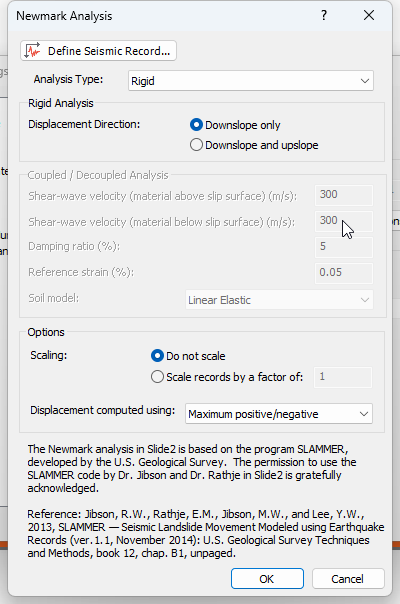
In this dialog, we can define the Newmark Analysis Type as either Rigid, Coupled, Decoupled, or All three. Displacements are computed by examining the Positive Acceleration, Negative Acceleration, Average (Mean) Acceleration, or Maximum positive/negative acceleration data points of the seismic record. All these accelerations can also be considered at once.

4. For this tutorial, we will use the default parameter values:
• Analysis Type = Rigid
• Displacement computed using = Maximum positive/negative acceleration

Next, we will import the Example record.

5. In the same dialog (shown above), click on Define Seismic Record and in the resulting dialog, click on Example Records.
6. In the Example Seismic Records dialog, select:
• Earthquake = Mammoth Lakes-1 1980
• Record Name = CVK-090.

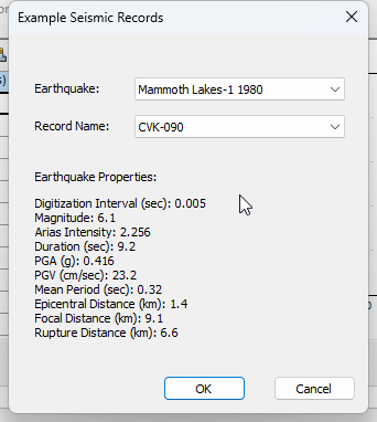
Notice that a summary of the Earthquake Properties, including the PGA and PGV of the selected record is displayed in the dialog.

7. Click OK to close the Example Seismic Records dialog.

The acceleration vs time plot is generated.

8. Click OK to close all open dialogs. The seismic loading symbol will now be displayed in the model’s top right corner. This symbol is the true acceleration graph we saw in Define Seismic Record dialog.
9. Just as before, run the analysis (Analysis > Compute) and view the results (Analysis > Interpret).

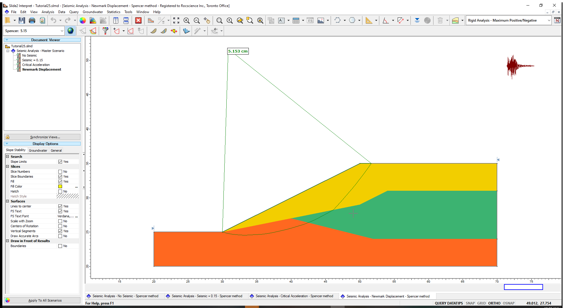
5.1 Computation and Interpretation of Results

The results show the critical slip surface with the highest Newmark displacement in cm.

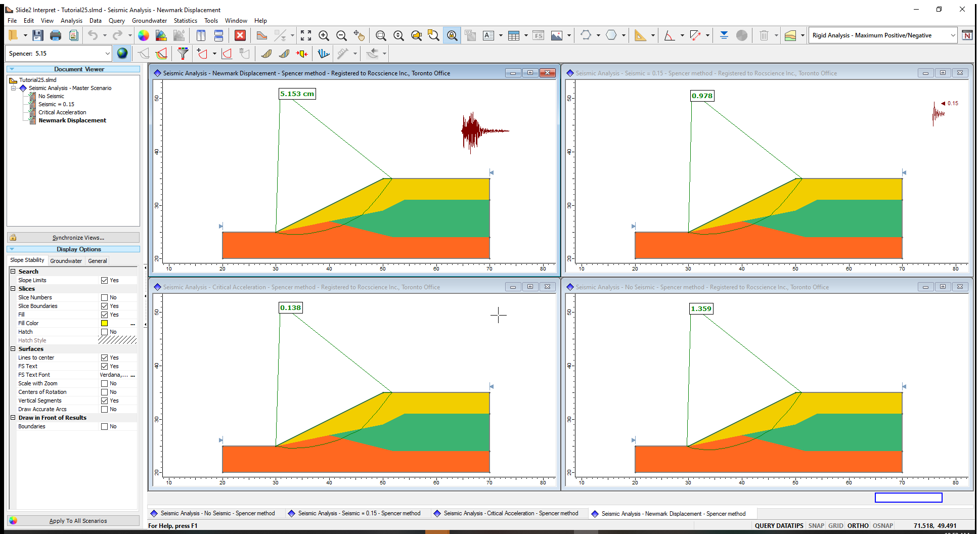
To easily compare the results:

1. Select Window > Tile Vertically
2. Minimize the master scenario which is the same as No Seismic scenario, and click Window > Tile Vertically again.
3. Below the Document Viewer pane, click Synchronize Views. Select the Sync Zoom/Pan/View Mode checkbox.
   
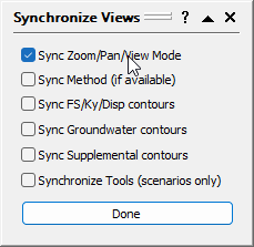
4. Select Done.

Once activated, this feature allows you to apply the zoom and pan settings used in one scenario across all scenarios. Use the Zoom options as necessary to achieve the desired view of the slopes.

This concludes the seismic analysis tutorial.

6.0 References

Jobson, R.W., Rathje, E.M., Jibson, M.W., and Lee, Y.W., 2013, SLAMMER – Seismic LandSlide2 Movement Modeled using Earthquake Records (ver.1.1, November 2014): U.S. Geological Survey Techniques and Methods, book 12, chap. B1, unpaged.