16 - Handling Tension in Limit Equalibrium

1. Introduction

In slope stability analyses with cohesive soils, tension forces may be observed in the upper part of the slope. In general, soils cannot support tension so the results of these analyses may not be very accurate.

In Slide2, there are a few ways to eliminate tensile forces in the slip surfaces.

In the first part of this tutorial, we will discuss using tension crack boundaries to obtain more accurate results. A tension crack essentially terminates the slip surface, thereby removing the tensile stresses from the calculations. Different methods of determining the depth of the tension crack are explained. In the second part of the tutorial, we will discuss some other methods that can be used to eliminate tension.

The completed tutorial file is Tutorial 16 Handling Tension.slmd, which can be found in File > Recent Folders > Tutorials Folder.

2. Model with No Tension Cracks

1. Start the Slide2 program.
2. Select File > Recent Folders > Tutorials Folder in the menu and open the starting file Tutorial 16 Handling Tension – starting file.slmd.

2.1 PROJECT SETTINGS

1. Select Analysis > Project Settings in the menu to open the Project Settings dialog and select the Methods tab on the left.
2. Notice that the Spencer method is selected. We need to use the GLE/Morgenstern-Price or Spencer analysis methods in order to obtain the thrust line (discussed later in the tutorial).
3. Click Cancel to close the Project Settings dialog.

2.2 COMPUTE AND INTERPRET

1. Select Analysis > Compute from the menu to perform the analysis.
2. Select Analysis > Interpret from the menu to view the results.

2.3 RESULTS

The factor of safety result is shown. For the Spencer (and GLE) methods we can plot a thrust line for the analysis.

1. Select Query > Show Line of Thrust from the menu.
2. Click Add Query.

The plot should look like this:

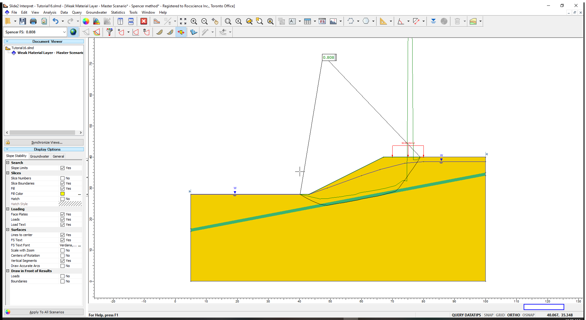
The thrust line gives the location of the resultant interslice forces (see Show Line of Thrust for more information). The important thing to observe here is that the thrust line extends outside of the sliding mass near the top of the slope. This generally indicates that tension is present.

To examine this further, we can view the force balance on each slice.

3. Select Query > Query Slice Data from the menu.

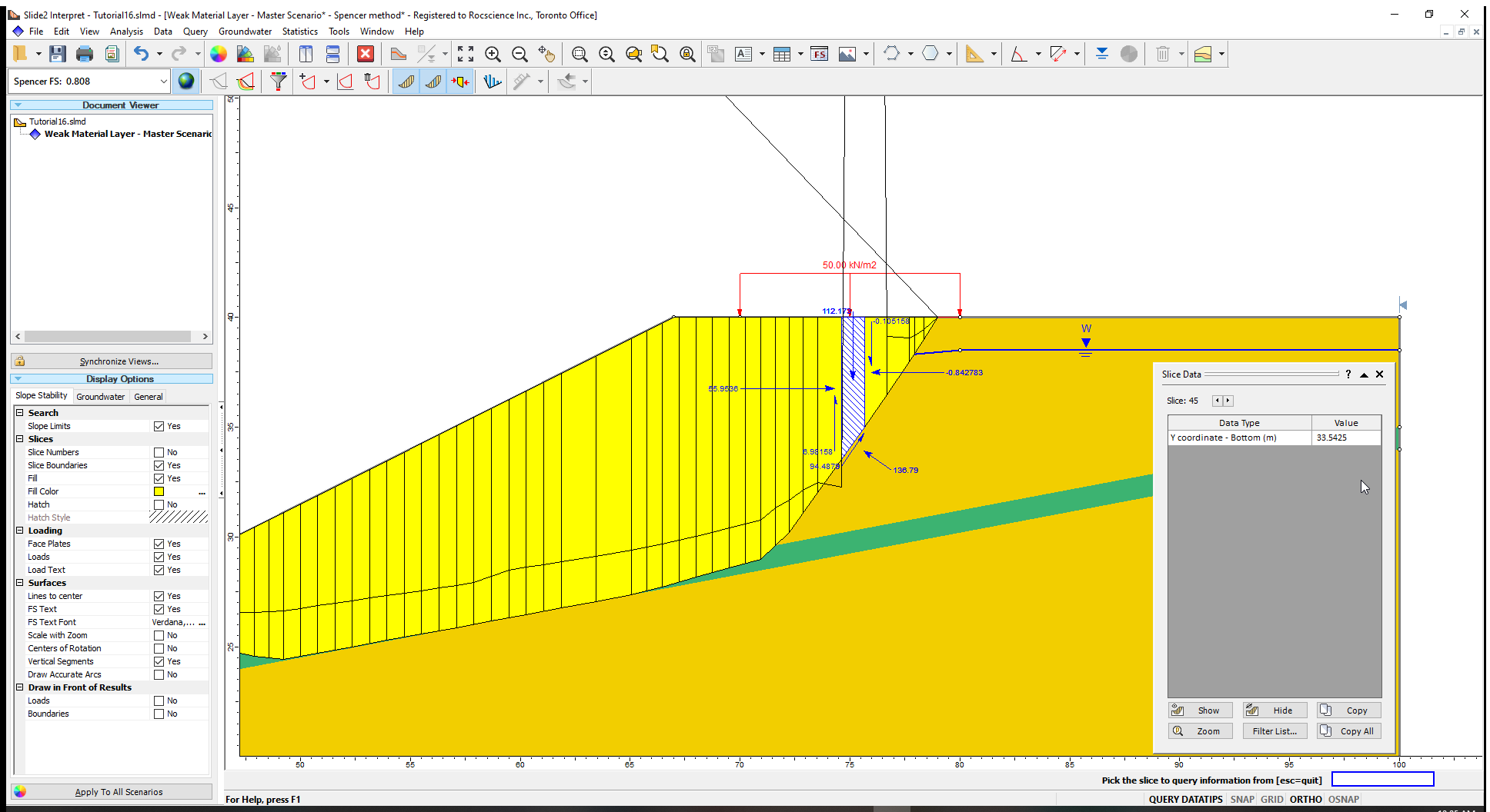
When you click on individual slices you can see the forces. For slices near the top of the slope you can see that the interslice forces are negative (note the minus sign in front of the force magnitude).

Click through the slices at the top until you reach the slice that shows negative forces on one side and positive forces on the other. This slice represents the transition from tensile to compressive interslice forces in the sliding mass. The location of the bottom of this slice can give a rough estimate as to the depth of the tension crack that will be required to eliminate the tension in the model.

While clicked on the slice that exhibits positive interslice forces on the left side and negative on the right side, scroll through the Slice Data and note down the “Y coordinate – Bottom (m)” value – we will call this D.

We can also graph the interslice forces to observe the tension.

4. Close the Slice Data dialog.
5. Right-click on the slip surface and select Graph Query from the popup menu (or select Query > Graph Query and select the slip surface with your mouse).
6. In the Graph Slice Data dialog, set the Primary Data to plot as Interslice Normal Force.
7. Click the Create Plot button.

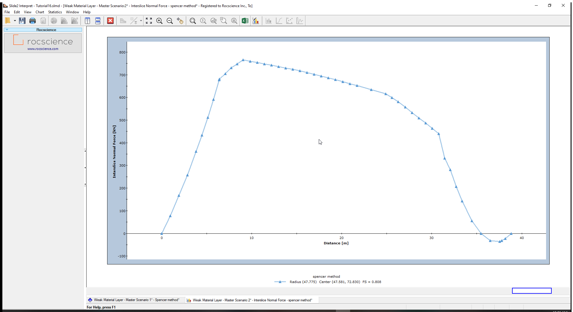
You should see the following graph. Notice the negative forces for the slices at the top of the slope. Also note that the absolute magnitude of the tension is relatively small, compared to the compressive forces further down the slope.

We will now rerun the model with a tension crack boundary to try to eliminate the tension.

3. Model with Tension Crack Boundary

1. Go back to the Slide2 Modeller program.

We now wish to eliminate the tension in the model. Duncan and Wright (2005, chapter 14) provide an informative discussion on tension in the active zone and describe how adding a tension crack can eliminate the effects of tension in the slope stability calculations. In Slide2, we can insert a tension crack boundary to delineate the lower extent of any possible tension cracks. The trick is to determine the depth at which to put this boundary.

As mentioned above, you could use the depth of the first slice in which tension is observed (y=D). Alternatively, analytical equations have been derived to determine the depth for a tension crack, for example, Abramson et al. (2002) give this relationship:

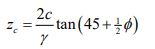
Where z_c is depth of tension crack, c is the material cohesion, φ is the angle of friction and γ is the unit weight of the soil material. This equation is derived in terms of effective stress parameters for a single homogenous material (although undrained strength parameters could also be used when appropriate). Use this equation and compare the value to D (from section 2.3).

We’ll add a new scenario to look at the effect of the tension crack.

2. Under Master Scenario, add a new scenario and name it “Tension Crack”. We will now edit this scenario.
3. To add the tension crack boundary, select Boundaries > Add Tension Crack in the menu.
4. Enter the right vertex (100, D).
5. We want the boundary to extend horizontally to intersect the slope, so right-click and ensure that Snap, Ortho and OSnap are all checked.
6. Close the context menu and draw a horizontal line that intersects the slope face.
7. Hit Enter to finish entering points.

You can see how the boundary delineates a zone of tension cracking. When a potential failure surface hits this zone, it will ascend vertically to the ground surface to create a tension crack.

By default, the tension crack zone is assumed to be dry. If the tension crack is set to be filled, then hydrostatic forces will be applied on the side of the slipping mass where it is terminated at the tension crack. A filled tension crack represents the worst-case scenario (it will give the lowest factor of safety). Since we want to compare this model to the original model with no tension crack, we will use the actual water table to define the crack saturation. To do this:

8. Right-click on the tension crack zone and select Tension Crack Properties.
9. For Water Level, select Use Water Table.
10. Click OK to close the dialog.

The model will now look like this:

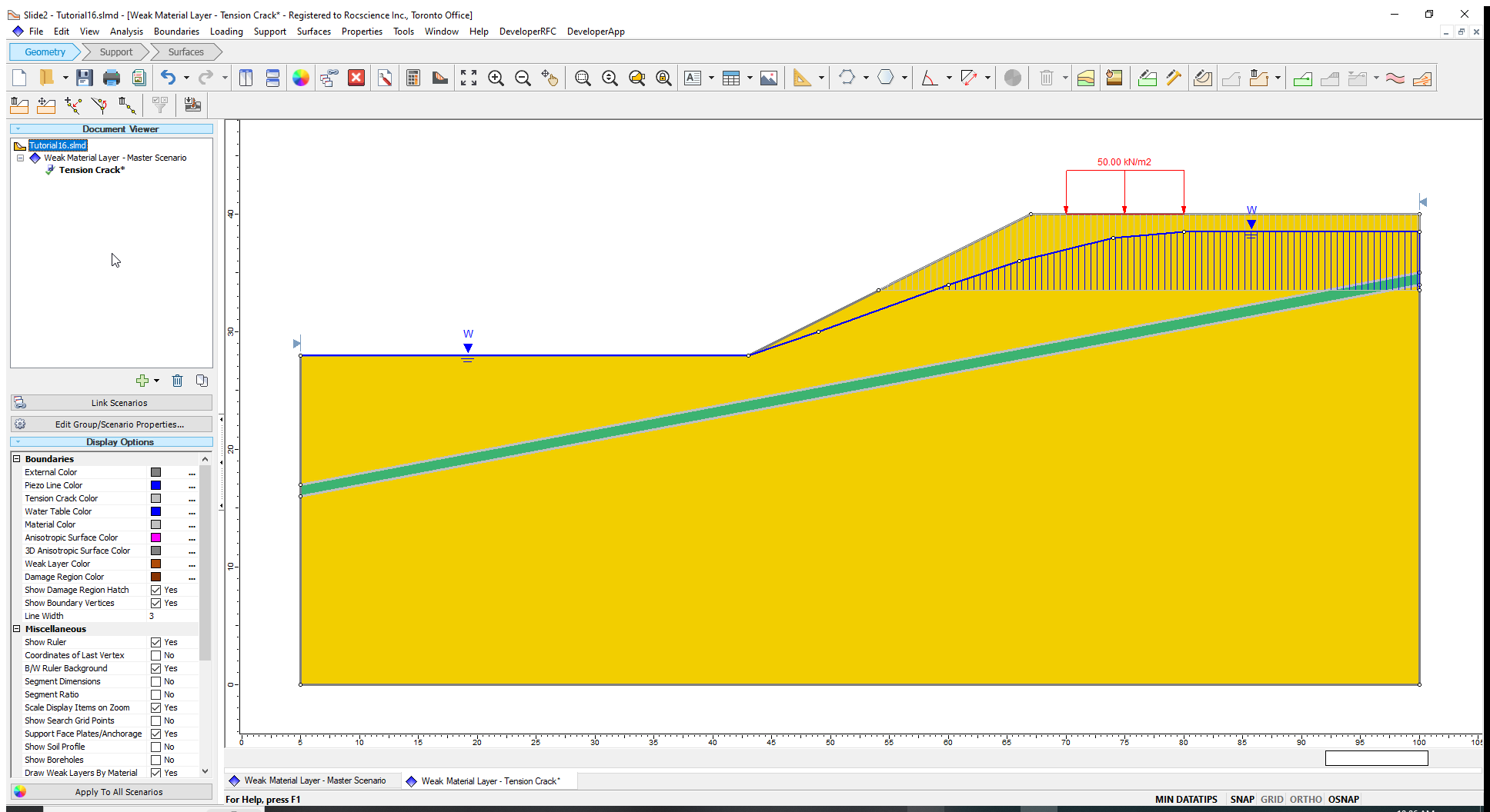
You can see how the potential tension cracks are now shown as saturated only up to the water table.

3.1 Compute and Interpret

1. Save and Compute (Analysis > Compute ) the model, then view the results in Interpret (Analysis > Interpret ).

3.2 Results

1. As before, add the thrust line (Query > Show Line of Thrust ). The results should look like this:

This plot shows several key differences from the example with no tension cracking:

• Where the failure surface intersects the tension crack boundary, a vertical tension crack forms that extends to the ground surface.
• The line of thrust is completely inside the failure surface indicating that there is no tension in the soil mass.
• The factor of safety has decreased slightly.

Although the difference in factor of safety is small, in general, it is good practice to introduce a tension crack zone for models which exhibit tensile interslice forces to obtain a more accurate failure surface and to eliminate possible numerical stability problems. For models with more extensive tensile zones or larger tensile forces, it may be essential to introduce a tension crack zone in order to obtain realistic results.

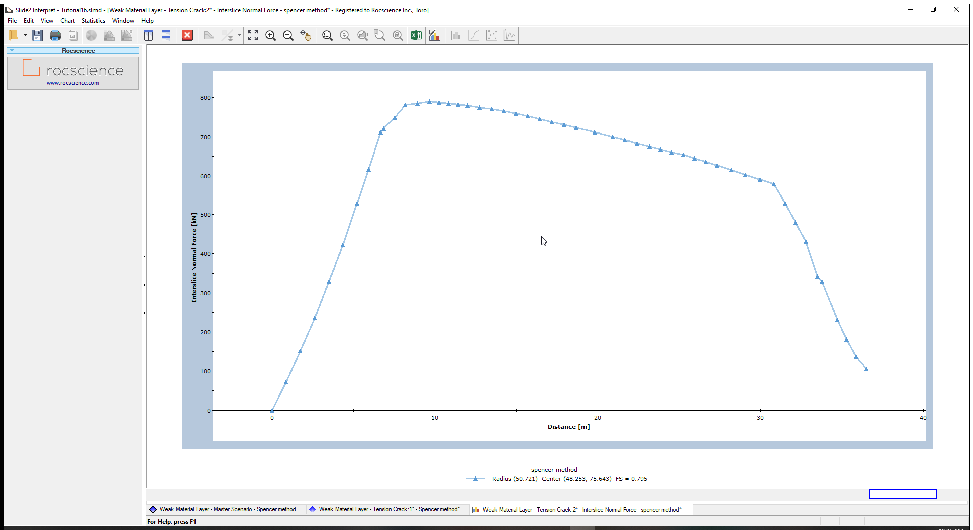
If we graph the interslice normal force as we did previously, the graph indicates compressive interslice forces for all slices with no tension present, as shown in the next figure. Note that the normal force on the last slice is not zero – this is due to the hydrostatic water force in the tension crack. If the tension crack zone were dry, the normal force on the side of the last slice would be zero.

4. Tension Crack Sensitivity Analysis

The tension crack depth used in the previous section eliminates the tension in the model and therefore produces more reliable results. There are many valid possibilities for tension crack depth that will eliminate the tension in the model. We now wish to determine the tension crack depth that minimizes the factor of safety. We can calculate this depth using a sensitivity analysis.

1. Go back to the Slide2 model program.
2. Add another child scenario and rename it Sensitivity.
3. Select Analysis > Project Settings from the menu.
4. Select the Statistics tab on the left and tick the checkbox for Sensitivity Analysis.
5. Click OK to close the dialog.

We will now define the upper and lower limits of the tension crack boundaries, and Slide2 will test 50 possible tension crack boundary locations in between these limits.

6. Select Statistics > Tension Crack > Draw Min Tension Crack in the menu.
7. Enter 100, 32 for the right coordinate.
   As before, ensure that all snapping is turned on by right-clicking and turning on all snap options.
8. Draw a horizontal line that intersects the slope surface (at 51, 32).
9. Hit Enter to finish entering points.

You have now defined the minimum (bottom) tension crack boundary.

To draw the maximum (top boundary):

10. Select Statistics > Tension Crack > Draw Max Tension Crack in the menu.
11. Click on the top right corner of the model (100, 40).
    Now, it is important that the top boundary extends the same horizontal distance as the bottom boundary.
12. To get the second point, move the cursor to the left point of the bottom boundary and hold it there for a moment but don’t click!
    You will now see a dashed red line extending vertically.
13. Move up the vertical line so that you are drawing a horizontal line. (Alternatively input (51, 40) in the prompt line.)
14. Hit Enter to finish entering points.

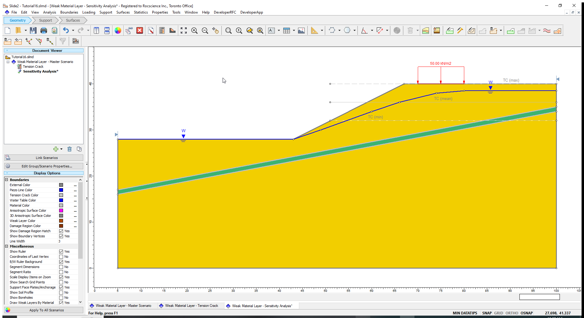
You will now see the minimum, maximum and mean tension crack boundaries as shown:

As before, we only want the tension crack saturated below the water table.

15. Select Properties > Define Tension Crack from the menu.
16. Set the Water Level to Use Water Table.
17. Click OK to close the dialog.

4.1 Compute and Interpret

1. Save the model by selecting File > Save in the menu.
2. Select Analysis > Compute from the menu to perform the analysis.
3. Select Analysis > Interpret from the menu to view the results.

4.2 Results

1. As before, add the thrust line (Query > Show Line of Thrust) and the results should look like this:

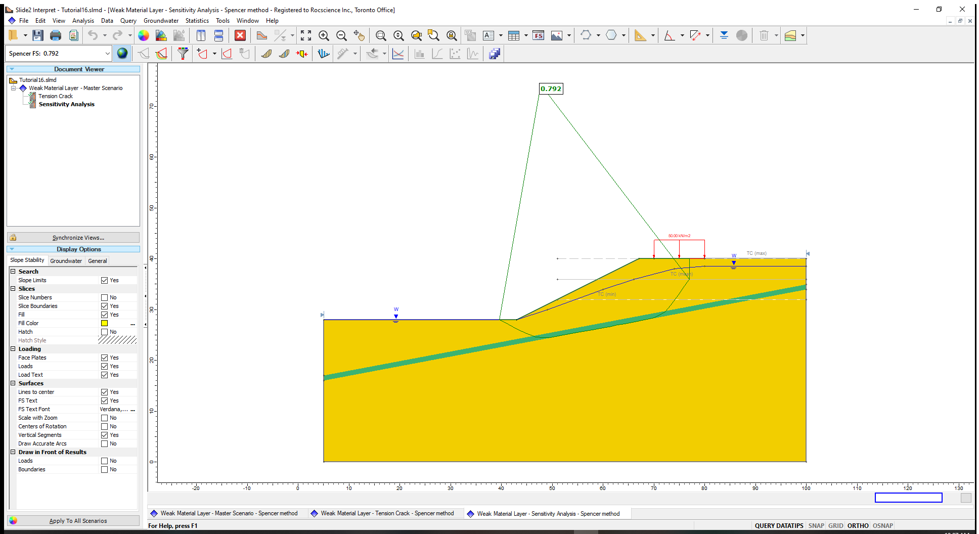
This plot is showing the results for the mean tension crack location. For the mean boundary (at a depth of 4 m), the thrust line is completely inside of the sliding mass indicating no tension.

To examine the results of the sensitivity analysis:

1. Select Statistics > Sensitivity Plot in the menu.
2. Choose the Spencer analysis method and, under Data to Plot, tick the check box for Sensitivity – Tension Crack Location.
3. Click the Plot button.

You will see the factor of safety plotted versus the tension crack boundary location.

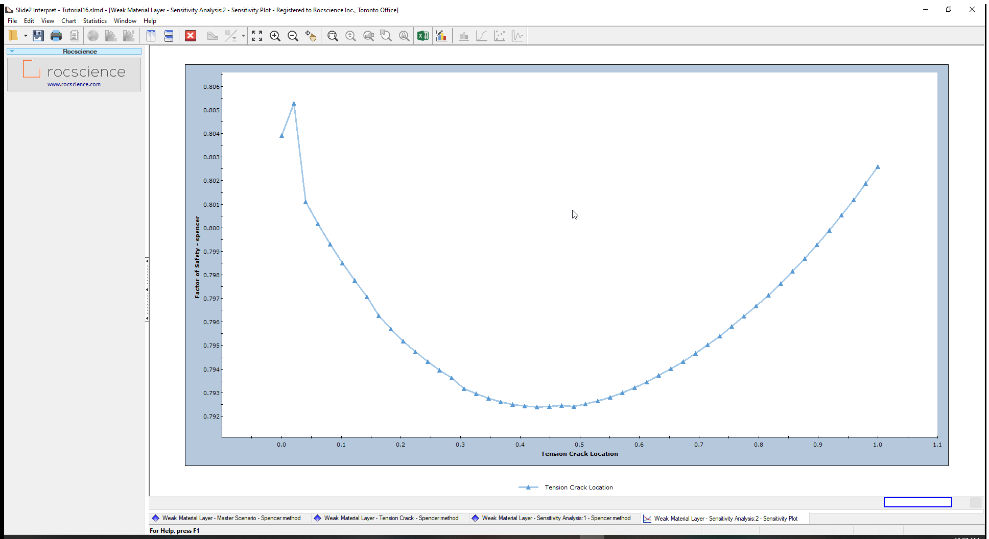
The tension crack boundary location is defined as a fraction of the distance from the minimum (32 m) to the maximum (40 m). The plot shows a clear minimum in the region between 0.4 and 0.5. This, therefore, corresponds to a y-coordinate between 35.2 m and 36 m.

To obtain more precise values from the graph, you can use the Sampler options. For example, right-click on the chart and choose the Sampler > Show Sampler option. Now hover the sampler on the lowest point of the graph.

To summarize, you can get a rough estimate of the tension crack depth using the depth of the slice where the interslice forces switch from positive to negative, or using Equation 1. With the sensitivity analysis you can obtain the depth that minimizes the factor of safety.

5. Alternative Methods for Handling Tension

The specification of tension cracks requires work to determine the tension crack depth. There are some alternative methods for handling tension in the model:

• Setting the Tensile Strength of the material to zero (via Properties > Define Materials). If this setting is applied and the base of a slice is in tension, then its shear strength will be adjusted to the value corresponding to the instance immediately prior to when the tensile strength is exceeded.
• In the Advanced Project Settings, the Tensile Stress Check can be used to eliminate slip surfaces if there is tension in any of the slices within a specified percentage of the slip surface from the toe.
• In the Advanced Project Settings, the Zero shear strength when base in tension option is checked by default, and prevents the evaluated shear forces on the base of the slice from becoming negative (it is recommended that this option is always ON).

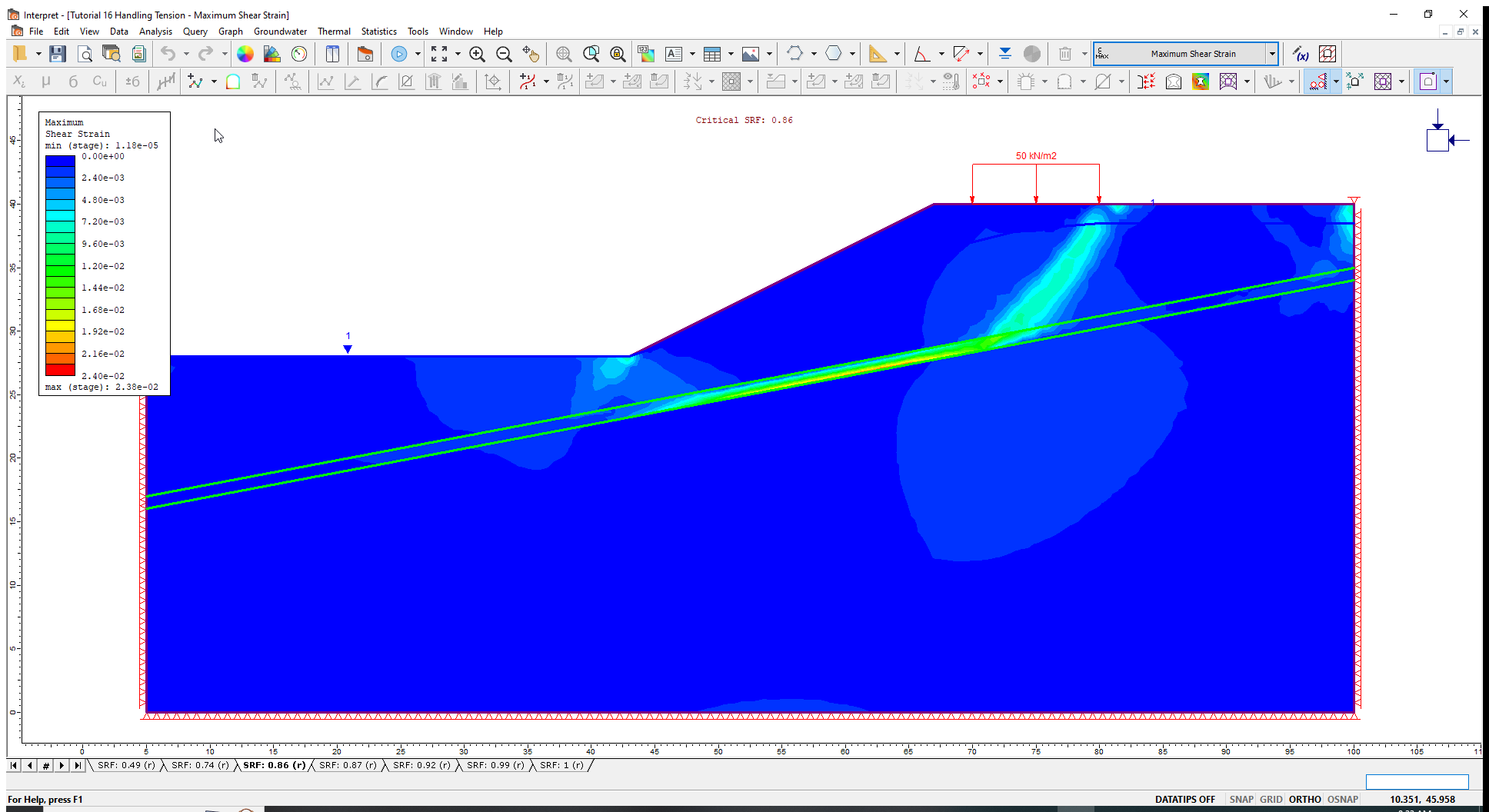
6. Optional Exercise in RS2

Drag and drop the model into RS2 and select the Master Scenario. Click Compute to compare the Limit Equilibrium results with Finite Element results.

7. References

Abramson, L.W., Lee, T.S., Sharma, S. and Boyce, G.M., 2002. Slope stability and stabilization methods, second edition, John Wiley & Sons Inc., New York.

Duncan, J.M. and Wright, S.G., 2005. Soil strength and slope stability, John Wiley & Sons Inc., New York.