2 - Materials and Loading
1.0 Introduction
In this Slide2 tutorial, we will determine the critical non-circular failure surface for an open pit slope with multiple materials. We will also model a groundwater table and an external load.
At the end of the tutorial, you will know how to:
- Create a Slide2 model by importing a DXF geometry cross-section
- Assign different material properties to the slope regions
- Specify pore pressure for the slope by using a water table
- Query the critical slip surfaces for detailed analysis such as base normal stresses and graph the results
The finished product of this tutorial can be found in the Tutorial 02 Multiple Materials and Loading.slmd data file. You can access tutorial files installed with Slide2 by selecting File > Recent Folders > Tutorials folder from the Slide2 main menu.
2.0 Project Settings
- Open a new Slide2 file and go to Analysis > Project Settings or click on the Project Settings
 icon in the toolbar to establish some primary settings for our model.
 - Under the General tab, change the Failure Direction to ‘Left to Right’ (This is because the critical failure surface of the cross-section moves in this direction). We will maintain the rest of the default options under the General tab.
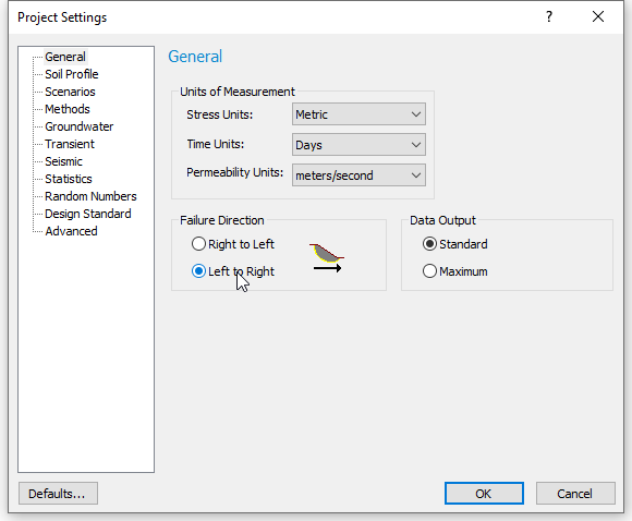
- Go to the Methods tab and uncheck any methods already selected. Select Spencer and GLE/Morgenstern methods.
- Select the Groundwater tab and set the Method to Water Surfaces. This method will be used to calculate the pore pressures that will develop in our slope model.
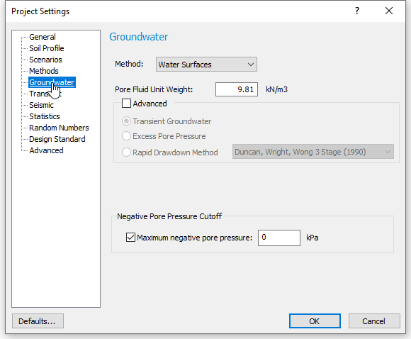
- Do not change any other settings. Click OK to close the dialog.
- Select Analysis > Project Summary
 and enter the title ‘Multiple Material Slope with Groundwater Table and External Loading’.
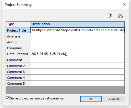
- Select OK to close the dialog.
Remember to save your work frequently.
3.0 Model
Our model comprises of:
- External Boundary
- Material Boundaries
We will create this by importing a DXF geometry cross-section.
- Select File > Import > Import DXF. A dialog for selecting and opening files will appear.
- Find and open the Tutorials folder (located in C:\Users\Public\Documents\Rocscience\Slide2 Examples).
- Select the file Geometry for Tutorial 02.dxf and click Open.
The model boundaries will be displayed and listed in the dialog shown below. Notice the selection of external and material boundaries in the left pane.
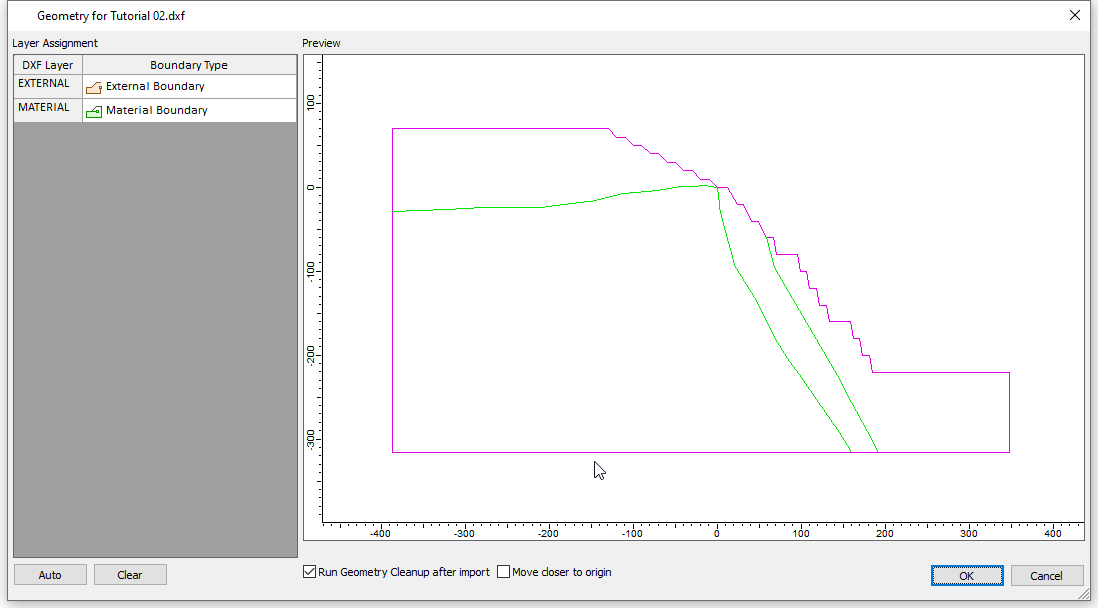
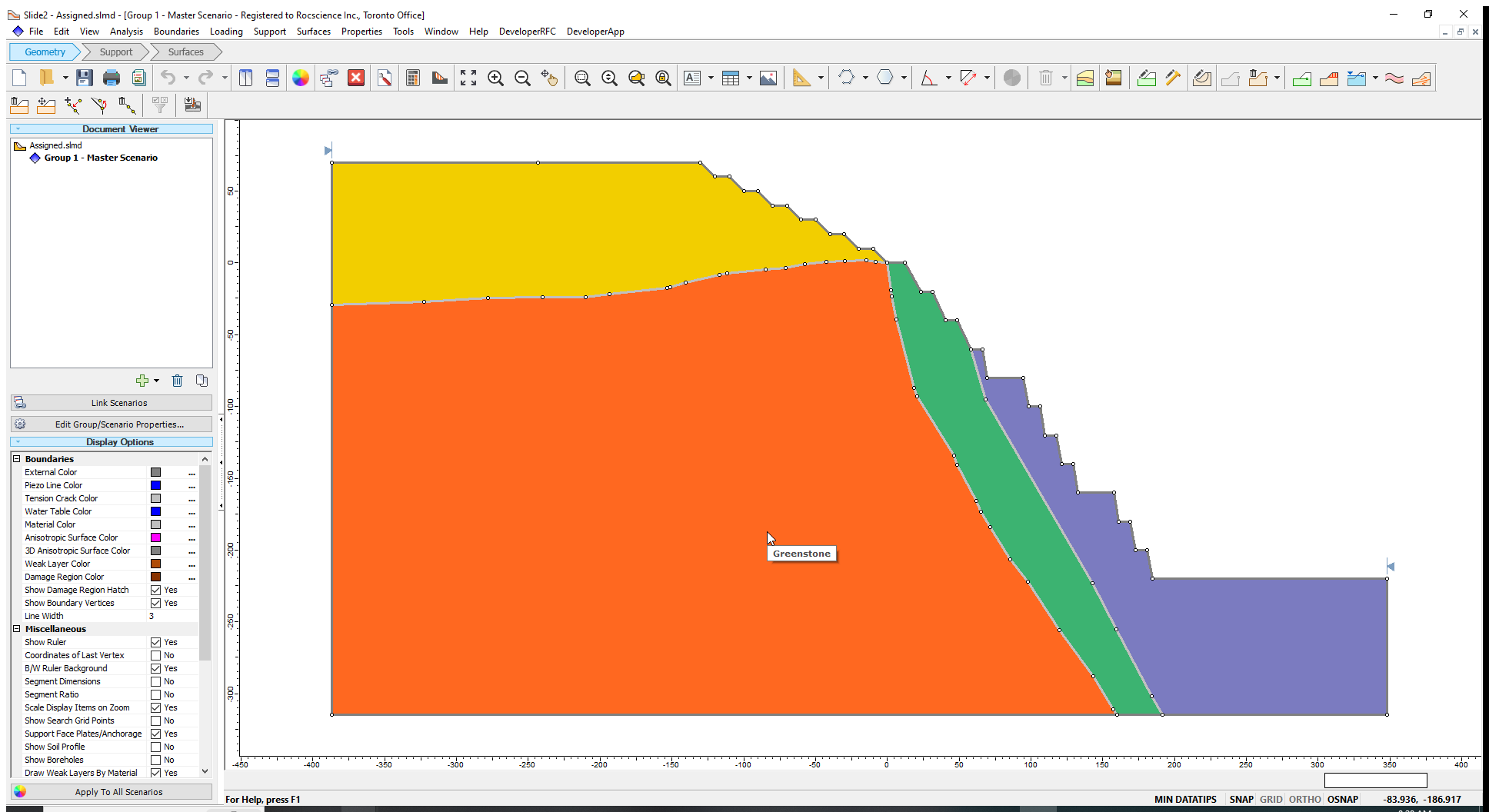
- OK to close the dialog. The model is shown below.
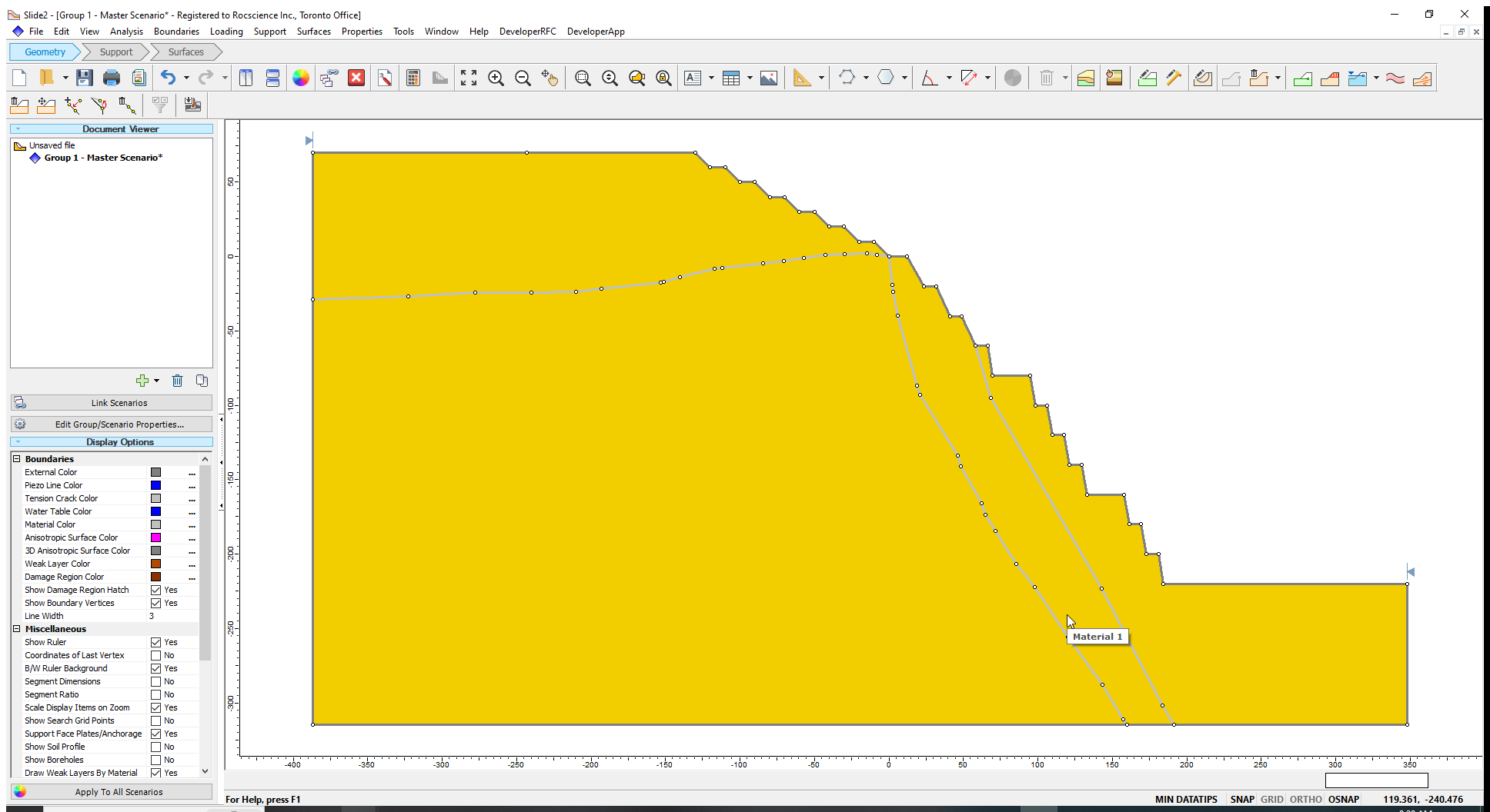
4.0 Material Properties
Our model has four different zones created by the external and material boundaries. The regions are automatically filled with the default material (Material 1).
By default, a newly created Slide2 file includes five materials, numbered from 1 to 5. We will:
- Rename the first four materials, and
- Define their strength properties in the material properties dialog
To define the material properties:
- Select Properties > Define Materials or click on the Define Materials
 icon in the toolbar.
 - Select Material 1.
Enter the following values for Material 1:
Name Saprolite Unit Weight 22 Strength Type Mohr-Coulomb Cohesion 20 Phi 30 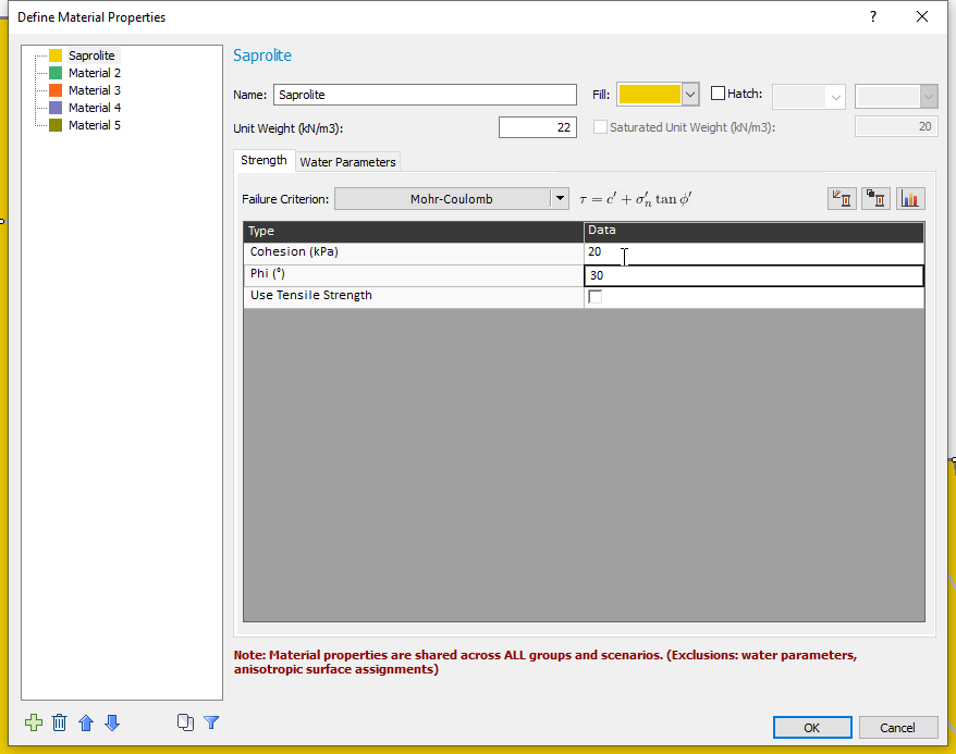
It is possible to change the fill colour to any colour of your choice, but we will use the default colours assigned to the materials for this tutorial.
As you did for Material 1 (the Saprolite), enter the name and material properties for the next three materials using values from the table below:
Material No. Material Name Unit Weight Strength Type UCS GSI mi D 2 Argillite 28 Generalized Hoek-Brown 50000 50 13 0 3 Greenstone 28 Generalized Hoek-Brown 200000 50 13 0 4 Tuff 28 Generalized Hoek-Brown 200000 50 13 0 - Click OK to close the dialog.
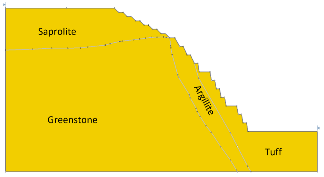
Now, we are going to assign the material properties to the slope regions indicated above.
- Select Properties > Assign Properties or click on the Assign Properties
 icon in the toolbar.
The Assign dialog will open and you will see a list of the material names we just defined.
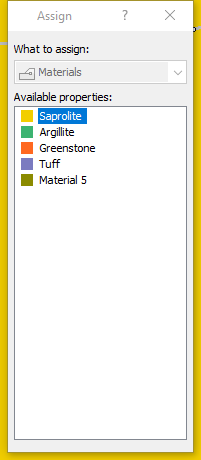
- Select the material name to be assigned to a zone from the list.
- Next, click anywhere within a zone to assign the material to that zone.
- Do this for all the model zones. Then close the Assign Properties dialog.
- You can assign a material property to a zone by right-clicking on a zone and selecting Assign Properties.
- To display different levels of data for materials, click the DATATIPS field below the command line. This action toggles between minimum or maximum data display on the model as you move the cursor across the regions.
5.0 Water Table
After assigning material zones, we will now define the water table for the slope.
- Select Boundaries > Add Water Table or click the Add Water Table Line
 icon.
icon. - Enter ‘t’ in the command line and press enter. This will generate a coordinate entry table.
Enter the water table coordinates in the table below.
X Y -405 36 -218 36 -151 28 -81 5 -5 -39 56 -84 133 -160 184 -220 410 -220 - Click OK to close the dialog.
- Press ENTER to finish editing.
Slide2 draws the water table. It also presents a dialog that allows you to specify the slope materials to which the water table applies.
We will assign the water table to all the materials, which is the default selection.
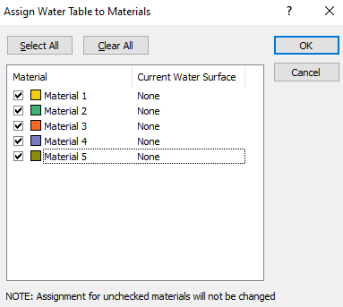
- Click OK to assign the water table and close the dialog.
6.0 Loading
We will apply an external load to the slope. In Slide2, external loads can be defined as concentrated line loads or distributed loads.
- Select Loading > Add Distributed Load
 to open the load dialog.
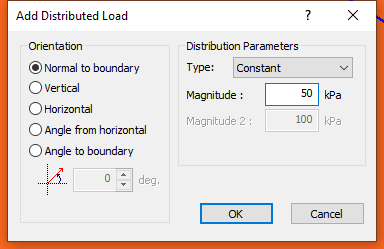
 - Enter the following parameters and click OK.
| Orientation | Distribution Parameters | |
| Normal to Boundary | Type | Magnitude |
| Constant | 50 | |
You may enter the location of the load graphically by left-clicking the cursor (which is now a red cross) at the desired starting and ending points of the distributed load. However, you can also enter coordinates for the start and endpoints.
For our tutorial, we will enter the following coordinates in the Prompt line:
(-243, 70); (-144, 70)
To do so:
- Enter -243, 70 into the Prompt line and press ENTER. You will notice the start point placed on the model.
- Next, enter -144, 70 into the Prompt line and press ENTER again. The endpoint will be added to the model.
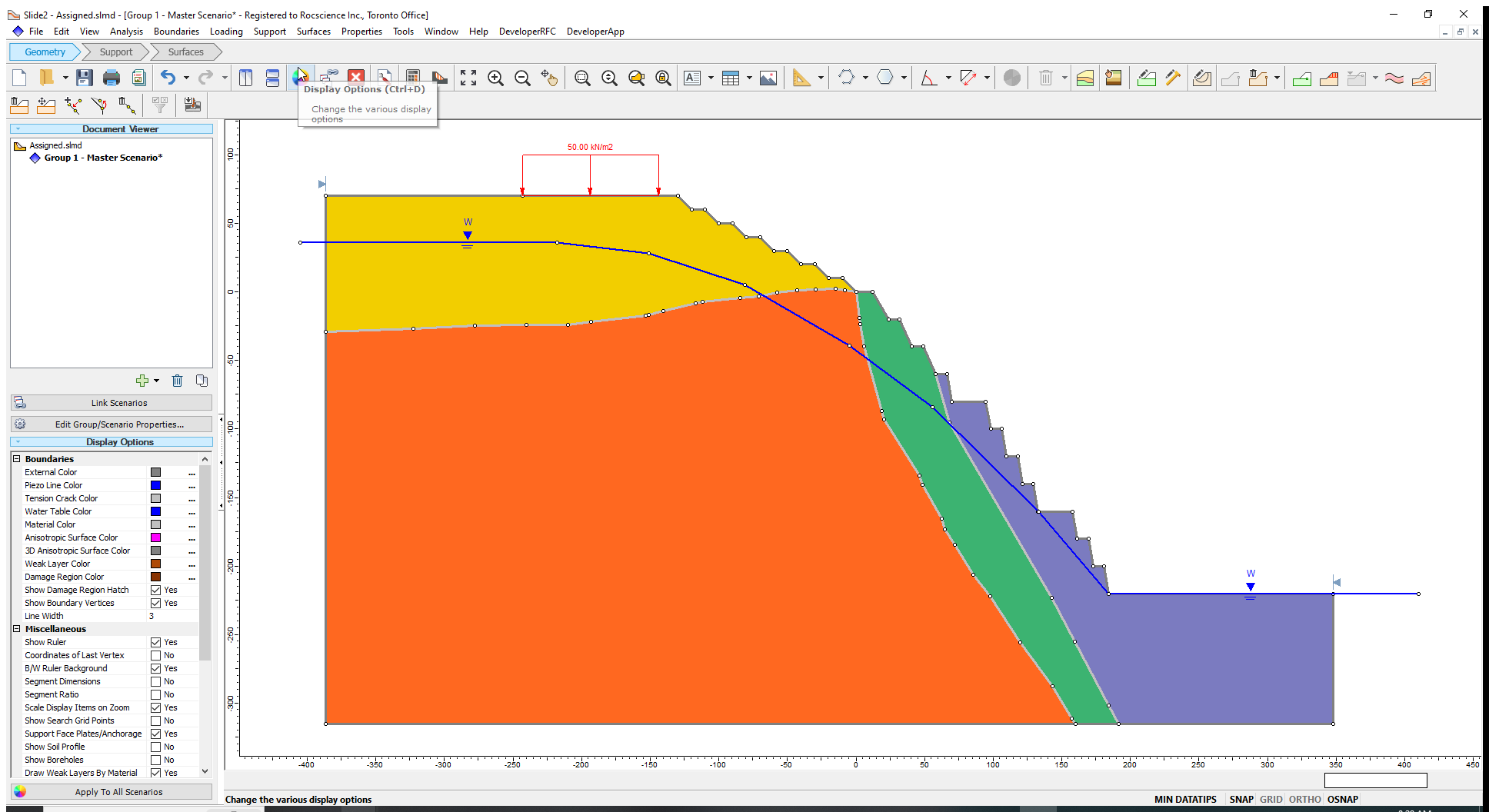
The distributed load is represented by red arrows pointing normal (downwards in this case) to the External Boundary, between the two points you entered. The load magnitude is also displayed.
7.0 Critical Slip Surface
In the Quick Start Tutorial, we used the Auto refine method to find the circular failure slip surface. This tutorial will explore non-circular failure surface analysis combined with a different search method - the Cuckoo Search method. This is the recommended search method in Slide2. You can explore the other search methods after this tutorial.
- Select Surfaces > Surface Options
 to open the dialog.
 - Set the Surface Type to Non-Circular.
- Ensure the Search Method is set to Cuckoo Search.
- Click OK to close the dialog.
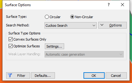
The Optimize Surfaces option, as its name suggests, allows Slide2 to optimally seek non-circular surfaces with factors of safety lower than a starting surface. The option applies local optimization to the surface found by Cuckoo to further refine the shape and Factor of Safety. It is recommended to keep this checkbox on.
Click here for more information on non-circular analysis and related search methods in Slide2.
We can now compute our model.
8.0 Compute
- Go to Analysis > Compute or click on the Compute
 icon in the toolbar.
Slide2's Compute engine will run the analysis and disappear when the computations are done. You are now ready to view the results in Interpret.
9.0 Results
- Select Analysis > Interpret or click the Interpret
 icon in the toolbar.
The Interpret window will open. Now we can view the results for our analysis.
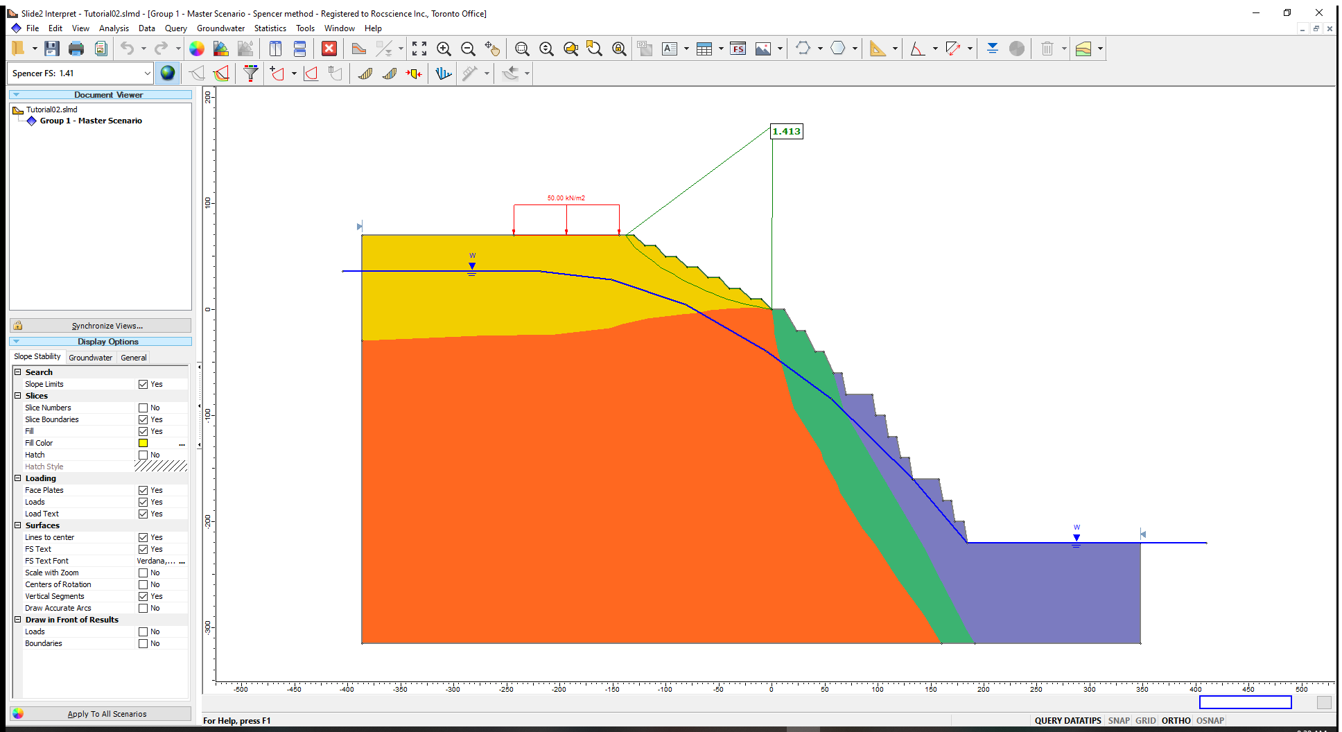
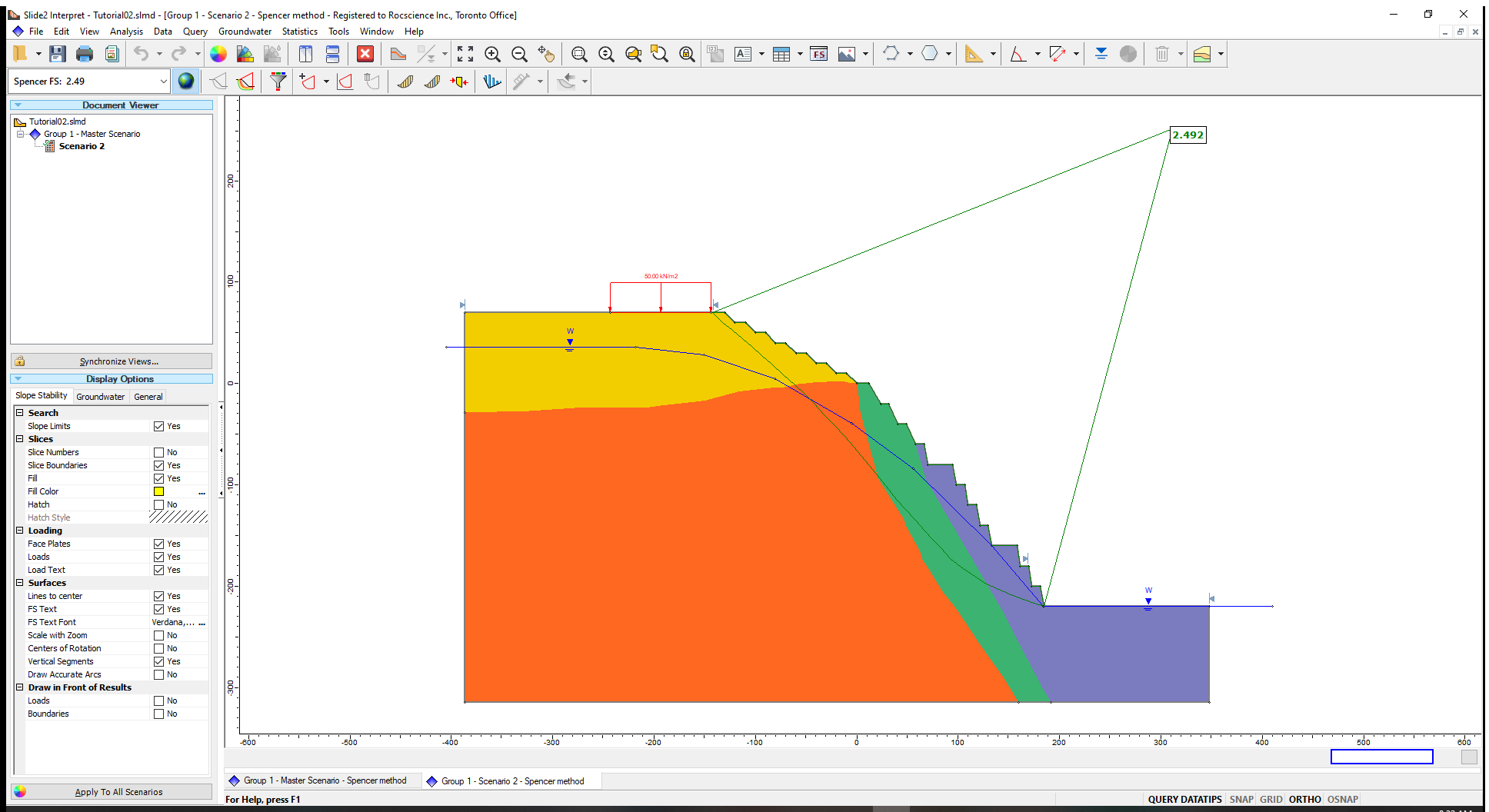
From our analysis:
- The factors of safety for both Spencer and GLE/ Morgenstern methods of analysis are approximately 1.4.
- The critical slip surface is localized to the Saprolite material.
The critical slip surface is localized to only the Saprolite region. However, let’s assume we want to evaluate the stability of other regions of the slope. We will create another scenario and use the double slope limits to evaluate the overall stability of the slope.
- Select Analysis > Modeller to return to the modeller.
In Slide2, the Multi Scenario modelling option is set as default under Project Settings. A Group consisting of a default Master Scenario is automatically created when you start a project. In this tutorial, we will create a copy of the Master Scenario, specify double slope limits, and then compute the new scenario.
To create another scenario:
- Right-click on the Group 1 Master Scenario, text in the Document Viewer on the left.
- Select Add Scenario.
A second scenario named Scenario 2 is created and listed in the Document Viewer.
- Click on Scenario 2 and set the double slope limits for the scenario by going to Surfaces > Slope Limits > Define Limits
 in the menu.
 - Select the checkbox for Second set of limits and enter the values shown below in the Left and Right data fields for the second limits:
- Left x coordinate:169
- Right x coordinate: 348
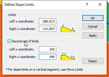
Two slope limits are now defined for our model.
button. The compute window will have Scenario 2 already selected since it does not have results.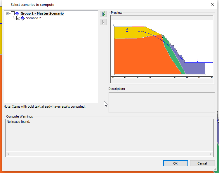
As expected, the factor of safety of the slope model in Scenario 2 is higher than the critical (localized value) in the Saprolite.
9.1 QUERY
Slide2 analysis gives us more than just the factor of safety and the slip surfaces. We will use the query feature in Slide2 Interpret to first view the base normal stresses for the overall slope slip surface and detailed analysis for individual slices in the sliding mass
- Go to Query > Add Query or click the Add Query
 icon in the Interpret window.
If you select Graph Query BEFORE you add any queries, Slide2 will automatically create a Query for the Global Minimum, and display the Graph Slice Data dialog. This saves the user the step of using the Add Query option.
- Select the overall critical slip surface or Global Minimum surface. If successfully selected, the surface colour changes from green to black.
These colours are set as the default in Slide2, and you can change them under Display Options.
- Go to Query > Graph Query or click the Graph Query
 icon.
icon. - Click on the drop-down arrow under Primary data and select Base Normal Stress.
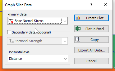
- Click Create Plot on the resulting dialog.
This action will close the dialog and open a new display tab in the Interpret window showing the graph of the Base Normal Stress of the slices below.
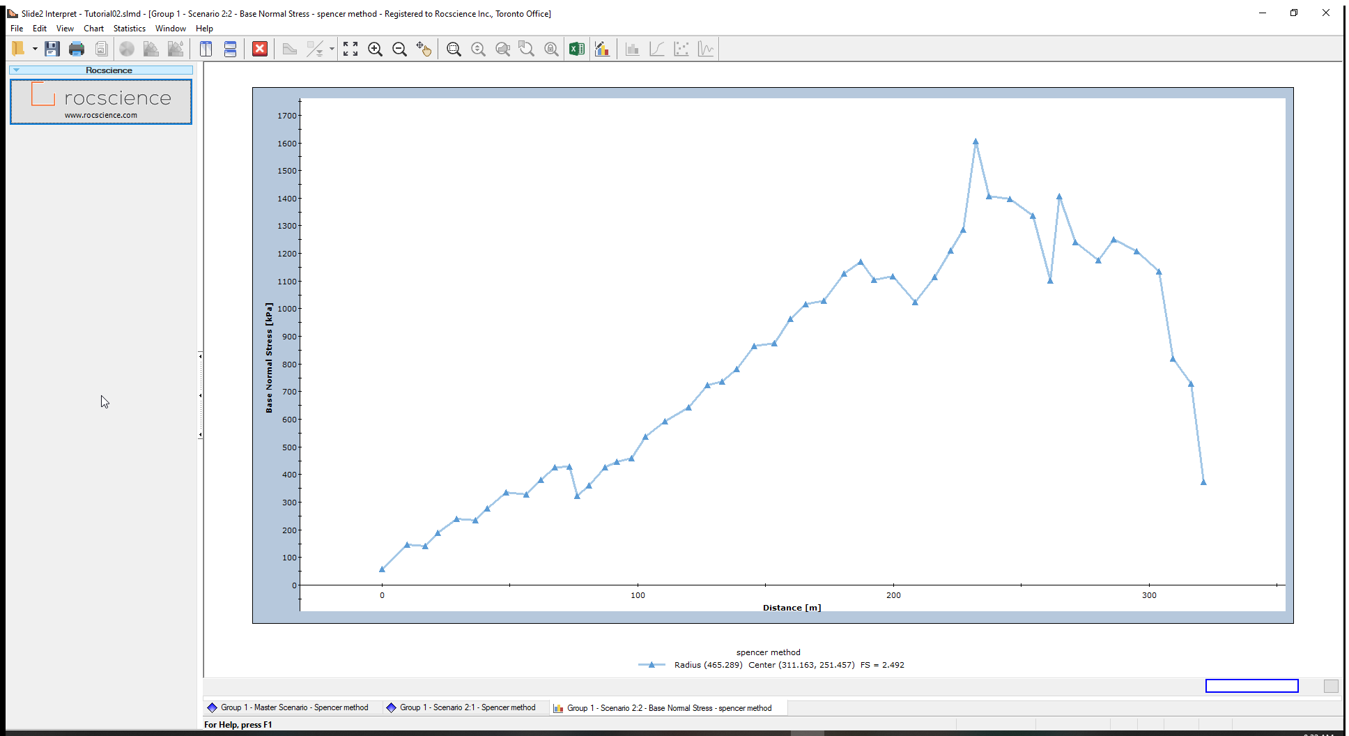
You can also edit properties of the graph such as the colour of the graph or font sizes of labels in the Chart Properties  dialog. You can use these graphs in your reports and presentations as well.
Close the graph view with the red X button  in the toolbar.
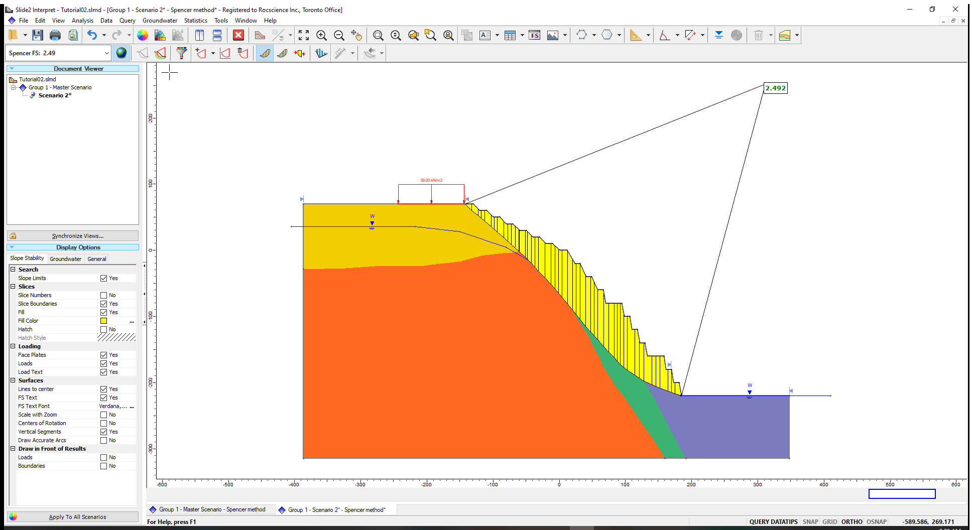
To view the slices:
- Select Query > Show Slices

The slices are immediately displayed on your model.
To see detailed analysis results for any slice:
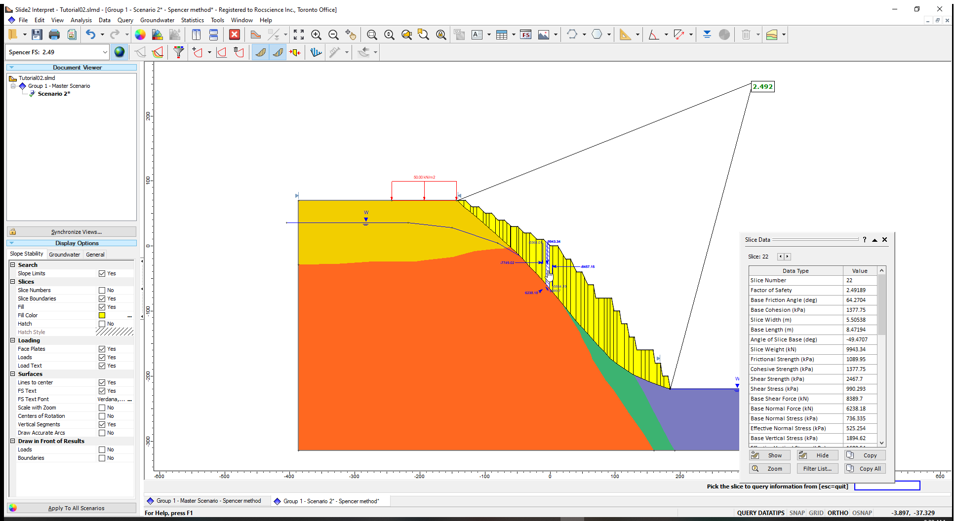
- Go to Query > Query Slice Data
 and select the slice of interest to see its properties.
An example is shown below.
This ends our tutorial.