4 - Finite Element Groundwater Seepage
1.0 Introduction
This tutorial will demonstrate how to model slope pore pressures using steady-state seepage Finite Element Analysis (FEA). Slide2 allows you to perform such an analysis using the same model developed for slope stability assessment (i.e., model geometry is defined only once and then used for both groundwater and slope stability analyses). The pore pressures, calculated from the finite element seepage analysis are automatically utilized in slope stability calculations. However, they can also be exported for use elsewhere.
Slide2 steady-state finite element analysis allows us to view groundwater results including:
- Contours of pore pressure, total head, and pressure head
- Flow lines, flow vectors, and isolines
In this tutorial, in addition to viewing the above-listed results we will also do the following:
- Use queries to obtain results at specific locations (lines, points, and boundaries) in the model and graph the results
- Query and graph the pore pressures along the Global Minimum slip surface
The finished version of this tutorial can be accessed in Tutorial 04 Finite Element Seepage Analysis.slmd by selecting File> Recent > Tutorials folder from the Slide2 main menu.
2.0 Geometry
We will use the file Tutorial 04 Finite Element Seepage Analysis - starting file.slmd as our initial model geometry.
- Select File > Recent Folders > Tutorials Folder.
- Open Tutorial 04 Finite Element Seepage Analysis - starting file.slmd.
2.1 PROJECT SETTINGS
To enable steady-state groundwater analysis, we will do the following in Project Settings:
- Select Analysis > Project Settings in the menu or click the Project Settings
 icon in the toolbar.
 - Under the Groundwater tab, set the groundwater method to Steady State FEA.
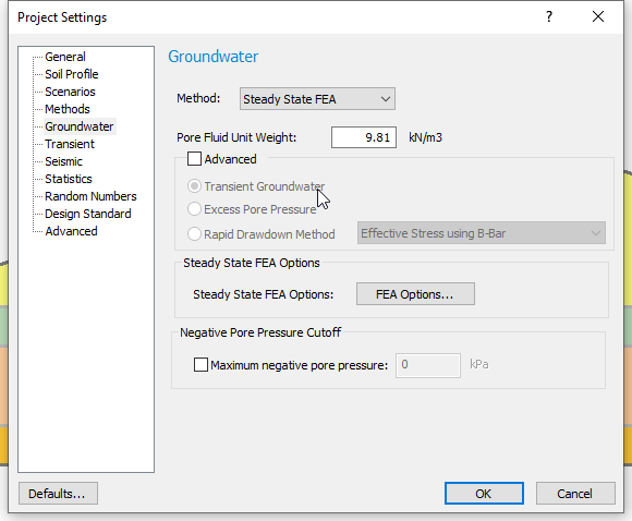
Project Settings Dialog - Click OK to close the dialog.
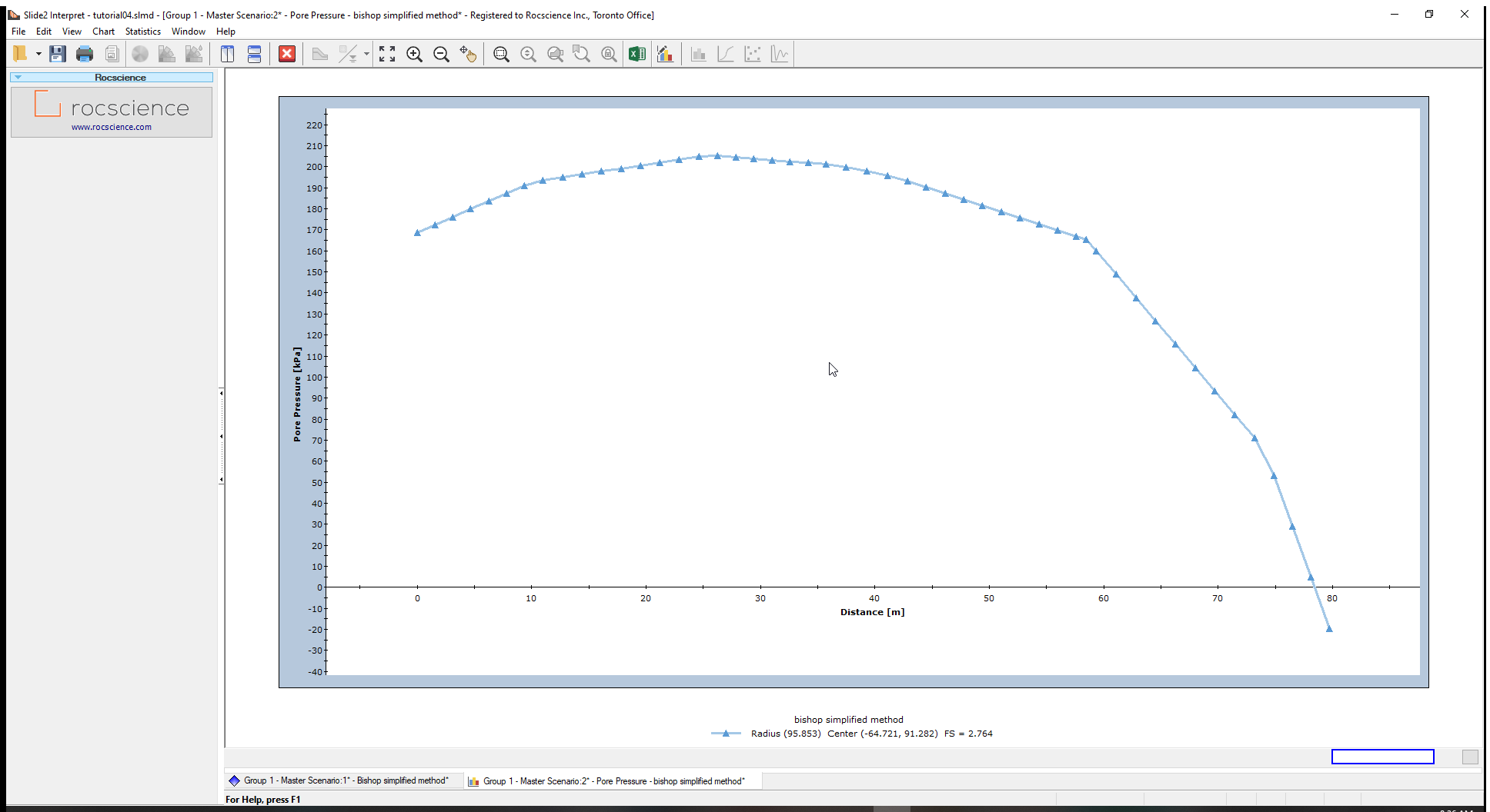
Two mode tabs - Slope Stability and Steady State Groundwater - appear at the bottom of the application window.
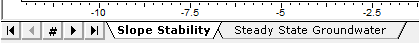
The Slope Stability analysis mode allows you to specify aspects of your model which are relevant to slope stability analysis, while the Groundwater analysis mode allows you to define boundary conditions and other settings relevant to groundwater analysis.
3.0 FEA Groundwater Modelling
- Click on the Steady State Groundwater tab.
When you are in the groundwater analysis mode, the menu and toolbar present the necessary Slide2 features required for finite element groundwater analysis.
For such an analysis, we will need to:
- Generate a finite element mesh
- Define boundary conditions
- Define the hydraulic properties (permeabilities) of the slope materials
3.1 MESHING
- Navigate to the Groundwater workflow tab

- Select Groundwater > Mesh > Discretize and Mesh in the groundwater menu or click the Discretize and Mesh
 icon.
icon.
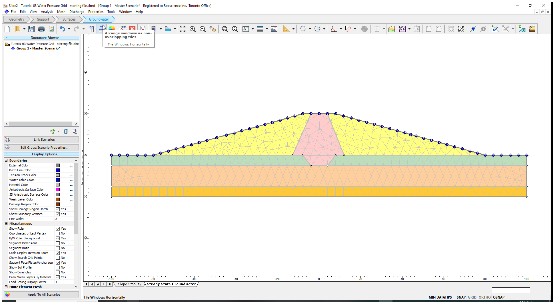
For this simple model, the default mesh generated by the ‘Discretize and Mesh’ option is adequate.
The simple mesh is generated based on the (default) Mesh Setup parameters specified in the Mesh Setup dialog. To view the parameters:
- Select Mesh > Mesh Setup or click the Mesh Setup
 icon in the toolbar.
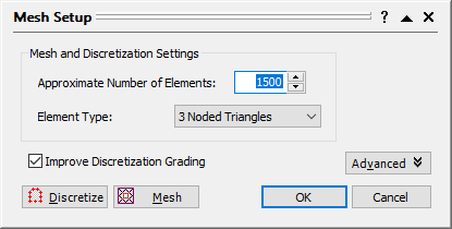
Although we will not modify these parameters in this case, Slide2 allows total user control over the generation and customization of the mesh. Close the dialog.
Refer to the Mesh and Mesh Options help page for more details on meshing in Slide2.
3.2 BOUNDARY CONDITIONS
After the finite element mesh has been generated, we must define all the necessary pressure and flow boundary conditions along the model boundaries. For our tutorial, we will define Total Head (H) boundary conditions. The upstream has a total head boundary of 17m and the downstream has a total head of 0m. These values represent known water levels at these locations.
- Navigate to the Groundwater workflow tab
- Select Groundwater > Mesh > Set Boundary Conditions or click on the Set Boundaries
 icon to open the dialog.
 - On the dialog, set BC Type as Total Head (H).
- Enter a Total Head Value of 17, which is the elevation of the phreatic surface (ponded water) on the upstream side of the model.
- Ensure the Selection Mode is Boundary Segments. (You can also use Boundary nodes or vertices. There are cases where they may be more convenient.)
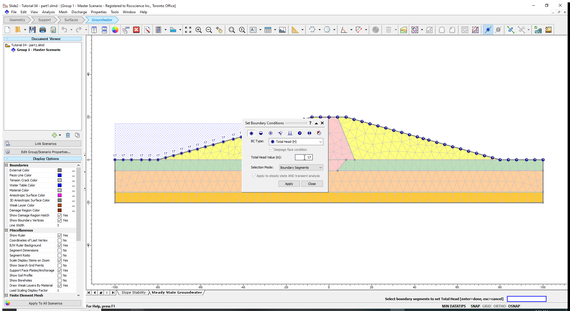
- Select the upstream segments (shown on the image above) and click Apply to assign the Total Head value of 17 as the boundary condition. Click Close.
Notice that the program automatically created a ponded water zone (the blue hatch pattern), corresponding to the Total Head boundary condition of 17 meters. This ponded water zone arises when Total Head values are greater than the elevations (y-coordinates) of an external boundary.
3.3 HYDRAULIC PROPERTIES
The last input we have to enter to complete the groundwater model is to define the hydraulic properties (permeabilities) of the slope materials.
- Select Properties > Define Hydraulic Properties or click on the Define Hydraulic Properties
 icon.
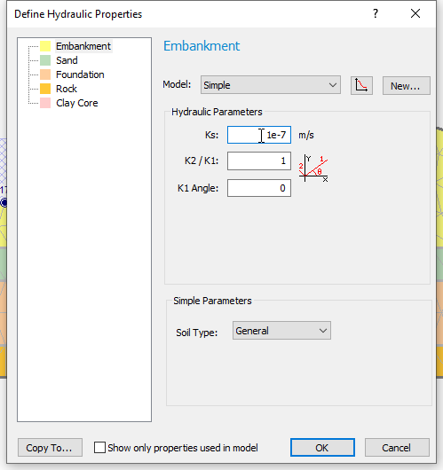
icon. Enter the following hydraulic parameters (Ks) for the slope materials.
Material Hydraulic Parameter (Ks) Embankment 1e-7 Sand 1e-5 Foundation 1e-8 Rock 1e-8 Clay Core 1e-9 We will maintain the default values for the Model, K2/K1 ratio and K1 Angle options.
- Click OK to close the dialog. We are now ready to compute the groundwater model.
- The groundwater analysis capability in Slide2 can be considered a completely self-contained groundwater analysis program and can be used independently of the slope stability functionality of Slide2.
- You may perform a groundwater analysis in Slide2, without necessarily performing a slope stability analysis.
- Although the Slide2 groundwater analysis is used for calculating pore pressures for slope stability problems, it is not restricted to slope geometry configurations. It can be used to analyze arbitrary, 2D groundwater problems undersaturated/unsaturated flow conditions.
4.0 Compute (Groundwater)
- Select Analysis > Compute (groundwater) or click on the Compute (groundwater)
 icon.
icon. - The dialog opens which indicates scenarios to be selected for computation. Ensure Group 1-Master Scenario is selected and click OK.
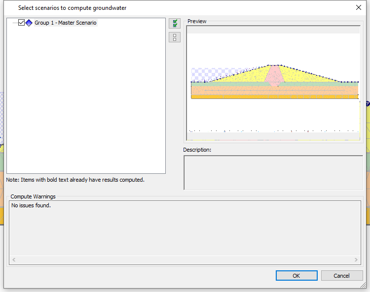
The groundwater compute engine will proceed to run the finite element seepage analysis. For this simple model, computations should only take a few seconds. When completed, you are ready to view the results.
5.0 Groundwater Results
We will view the following results:
- Pressure Head contours
- Total Head contours
- Pore Pressure contours
- Flow vectors
- Flow lines
- Iso-Lines
- Select Analysis > Interpret (groundwater) or click on the Interpret Groundwater Results
 icon .
5.1 PRESSURE HEAD CONTOURS
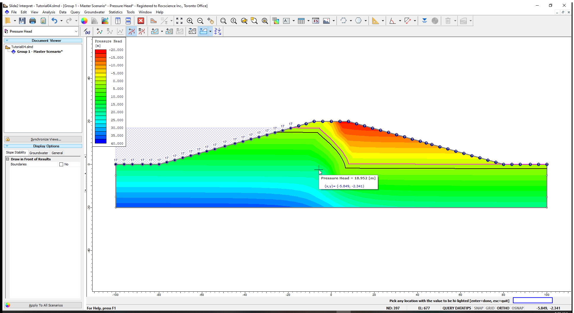
By default, Pressure Head contours are displayed. The Legend in the upper left corner of the view indicates the range of values.

The pink line (a default colour) displayed on the model represents the location of the phreatic surface (Water Table) determined from the finite element analysis. By definition, a phreatic surface is defined by the Pressure Head = 0 contour line.
5.2 TOTAL HEAD CONTOURS
Select Total Head from the contour display dropdown to view those contours.
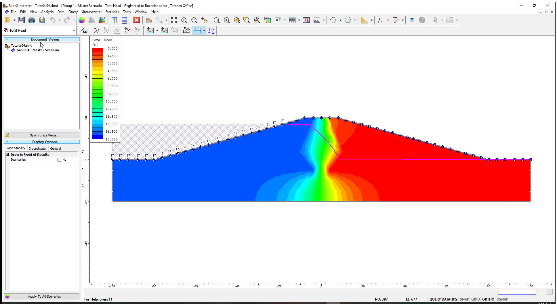
The Total Head values for the upstream side of the model are 17 as specified for the boundary conditions. The steep Total Head gradient (drop) across the embankment core is depicted by the rapid change in contour values.
5.3 PORE PRESSURE CONTOURS
In Tutorial 03, pore pressures were interpolated from the water pressure grid values, while in the current finite element seepage analysis, pore pressures are interpolated from the nodes of the finite element mesh.
- Select Pore Pressure from the dropdown in the contour display option to view the pore pressure contours.
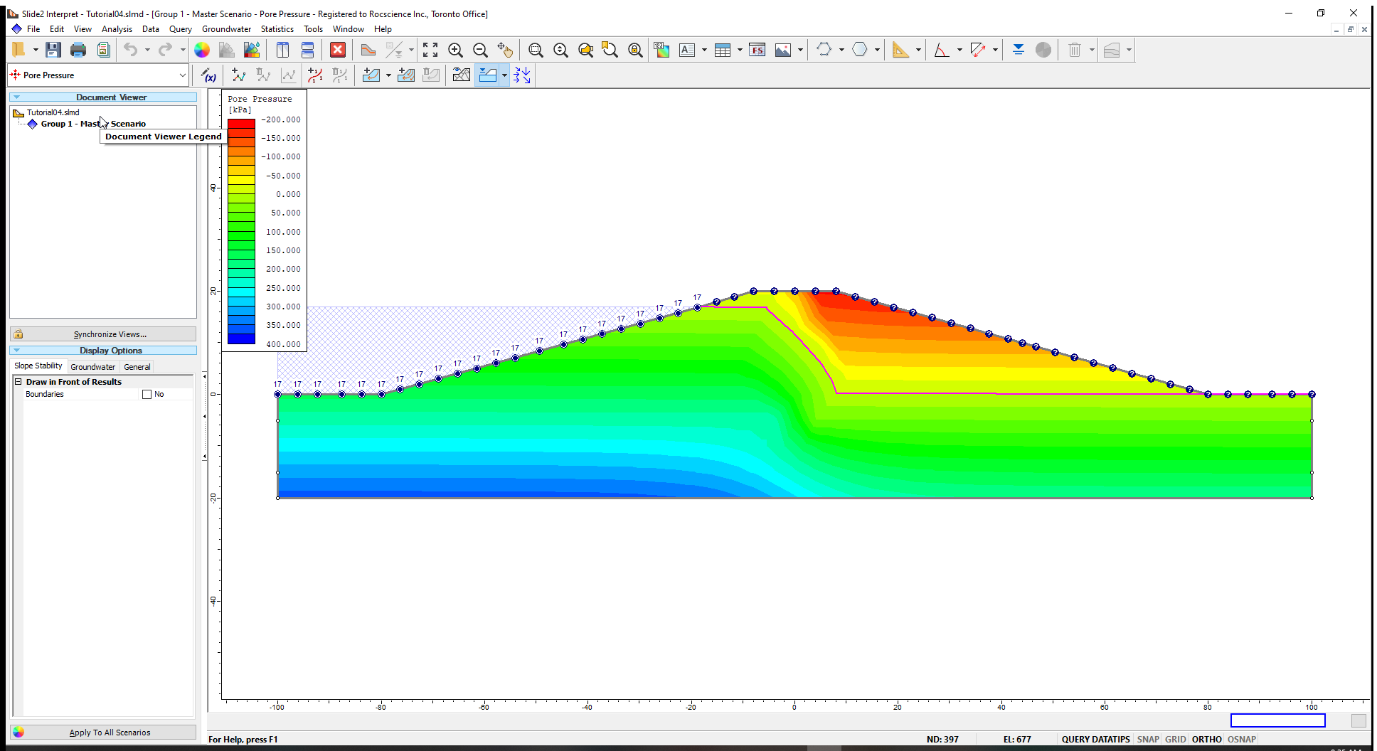
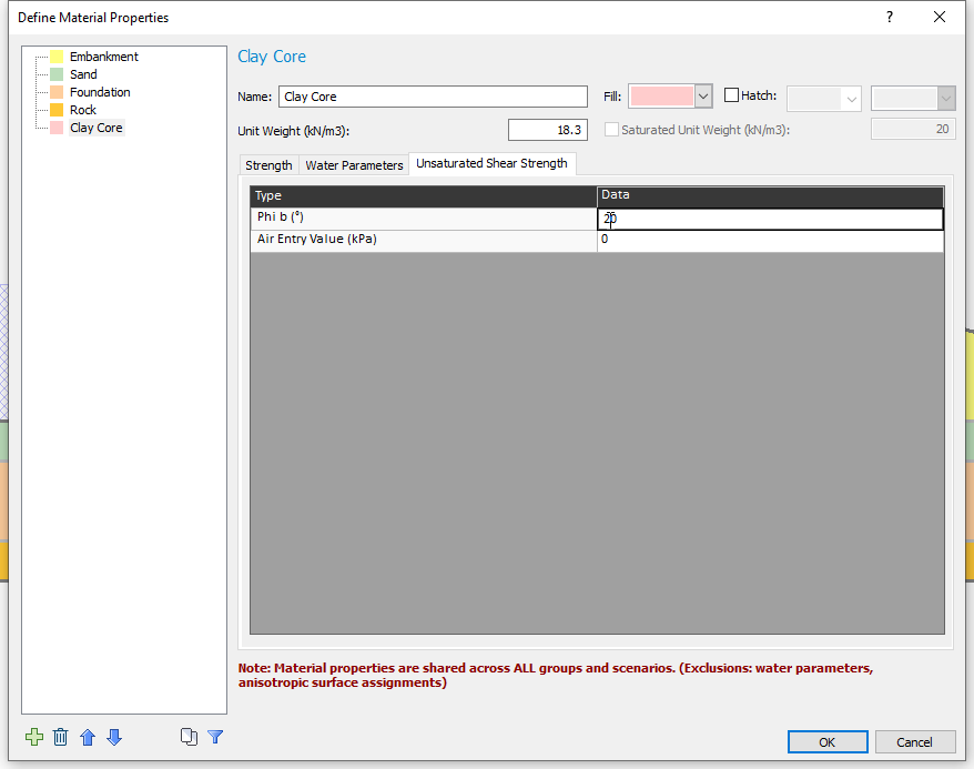
The unsaturated zone above the water table has negative pore pressures also referred to as ‘matric suction’. Matric suction contributes to the stability of a slope when unsaturated shear strength angle is specified for a material (or materials); it leads to INCREASED shear strength and higher safety factors.
By default, the Unsaturated Shear Strength Angle is set at 0. This means that matric suction in the unsaturated zone, WILL NOT have any effect on the shear strength or safety factor.
Click the Unsaturated Shear Strength help page to see more information on Unsaturated Shear Strength.
5.4 FLOW VECTORS
- We will now view the flow vectors by clicking on the Flow Vectors
 icon in the toolbar

You can toggle the flow vectors off by clicking on the Flow Vectors icon again (or uncheck the option in the Display Options dialog).
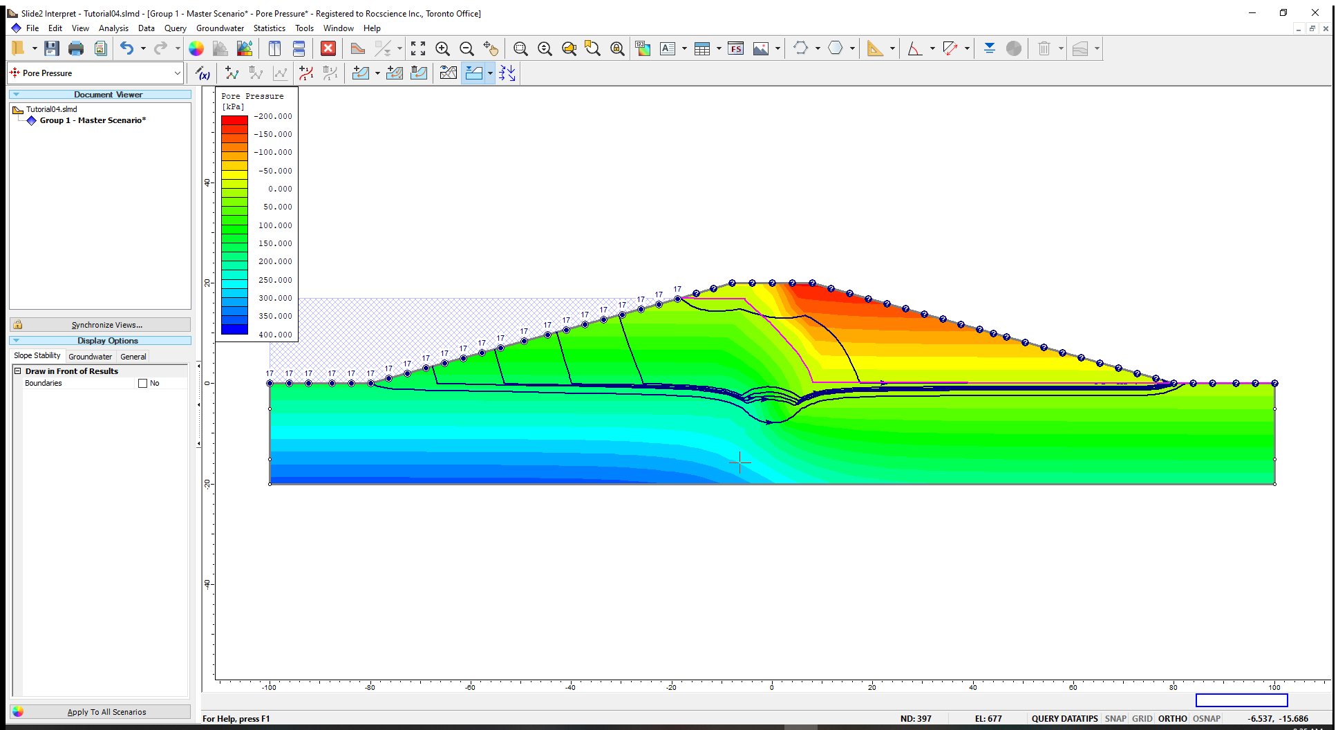
5.5 FLOW LINES
Flow lines indicate paths of the groundwater seepage from one point to another. They can be added individually or in multiples. We will use the Add Multiple Flow Lines option for this tutorial.
Ensure the Snap option in the Status Bar (underneath the command line) is enabled. (Alternatively, you can select View > Snap, and enable Snap from the popup menu if the mode needs to be activated). We are doing this to make it easier to select model vertices.
- Select Groundwater > Lines > Add Multiple Flow Lines or click on the Add Multiple Flow Lines
 icon.
icon. - Click the crest (-18.125, 17) and toe (-80, 0) of the upstream face of the embankment dam.
- Press Enter (or right-click and select Done) to open the dialog below.
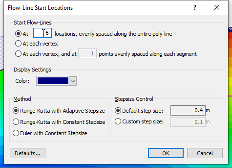
We will space our flow lines 6 evenly spaced locations. - Enter a value of 6 in the location's input box and click OK.
Your screen should look as follows:
Flow lines can be deleted in the manner indicated below.
- Click on the Delete Flow line
 icon.
icon. - Select the flow lines you want to delete, and press Enter.
5.6 ISO-LINES
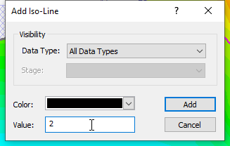
An iso-line is a line of constant value displayed on a contour plot. We will view the isoline for a pressure head value of 2, as an example.
- First, select Pressure Head Contours in the contour display box.
- Select Groundwater > Lines > Add Iso Line or click the Add Iso-Line
 icon.
icon. - Click anywhere on the model to open the Add Iso-Line dialog shown below.
- Enter a Pressure Head of 2.
- For this tutorial, ensure the colour is black for easy visibility of the iso-line.
- Click Add (or press Enter) to close the dialog.
The Iso-line is seen on the image below.
You can delete iso-lines with the Delete Iso-Lines  button.
TIP: Whenever a dialog has a question mark (?) on the top, you can click on it to access help information.
5.7 QUERIES
A query allows users to view exact values at specified locations.
We will create a query by drawing a vertical line from the upstream crest to the bottom boundary of the model.
- Select Groundwater > Query > Add Material Query or click on the Add Material Query
 icon.
icon. - Click on the vertex with coordinates (-8, 20) at the upstream crest of the embankment.
- For the second point, enter the coordinates (-5, -20) in the prompt line. (If you have the Ortho Snap option enabled, you can select this point graphically).
- Right-click and select Done or press Enter. You will see the following dialog:
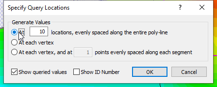
- Select the first radio button, enter a value of 10 in the locations input box, and ensure the Show queried values box is checked. Click OK.
The values for the 10 evenly spaced query points will be displayed along the vertical line.
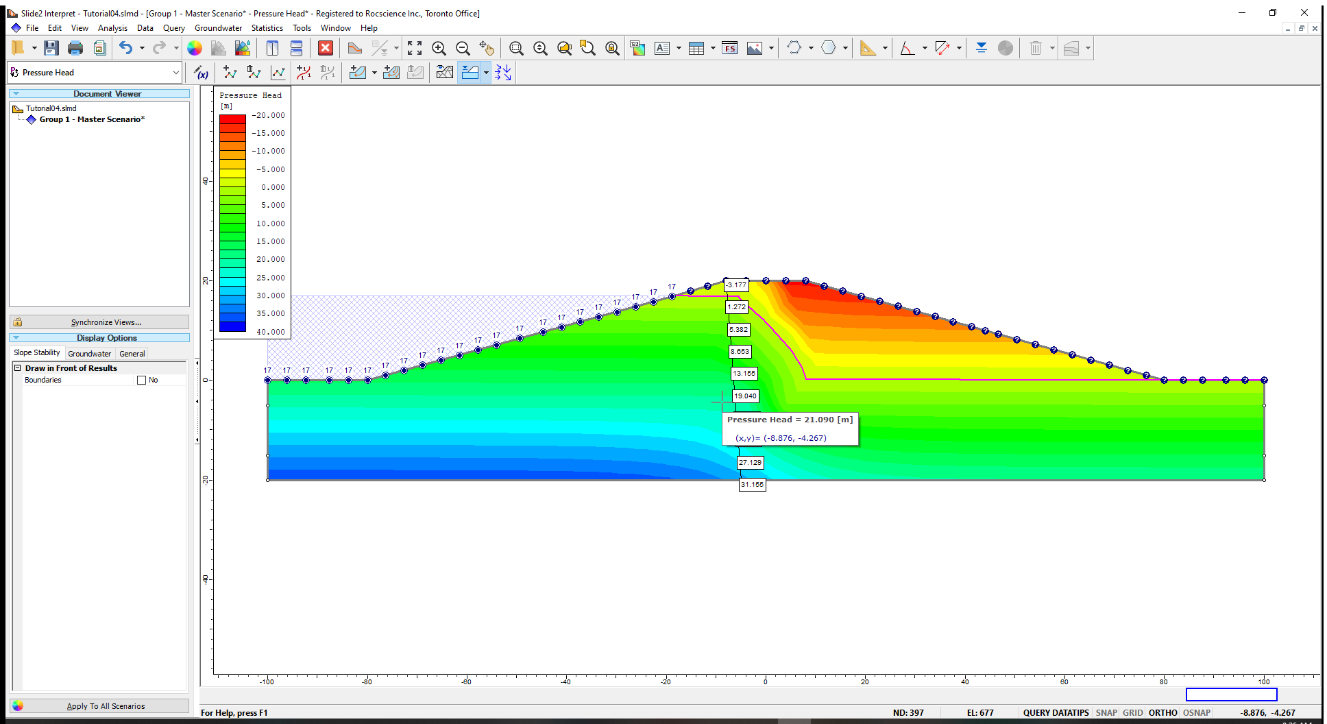
We can graph this data by simply right-clicking on the query line and selecting Graph Data from the resulting pop-up dialog.
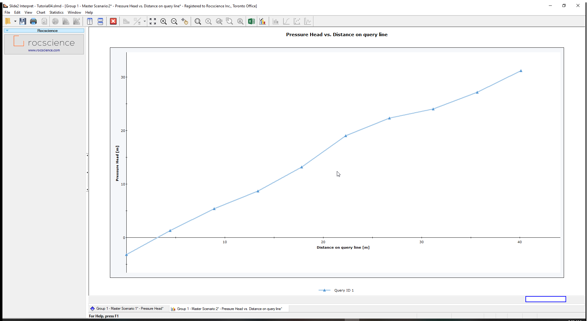
A graph of the pressure head values shown in the figure above will be generated in another window. Close the graph from the tab at the bottom, or by using the red X button in the toolbar.

6.0 Slope Stability Analysis
We will now evaluate slope stability using the pore pressures generated by the finite element seepage analysis. To return to the modeller:
- Select Analysis > Modeller or the Modeller
 icon in the toolbar.
 - Click on the Slope Stability tab.
The modelling toolbar options applicable to slope stability analysis in Slide2 are again displayed, and the groundwater features such as mesh and boundary conditions are now hidden.
6.1 COMPUTATION AND INTERPRETATION
- Select Analysis > Compute or click the Compute
 icon. The slope stability analysis will be conducted automatically incorporating the pore pressures calculated in the groundwater analysis.
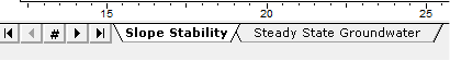
 - Select Analysis > Interpret or click the Interpret
 icon to view the slope stability results.
The factor of safety for the critical slip surface is approximately 2.8.
You will notice that the groundwater data contours are also displayed on the model.
You have the option to view only the Slope Stability results if you click on the drop-down arrow beside the  icon and turn off Groundwater mode.
6.2 PORE PRESSURE GRAPH
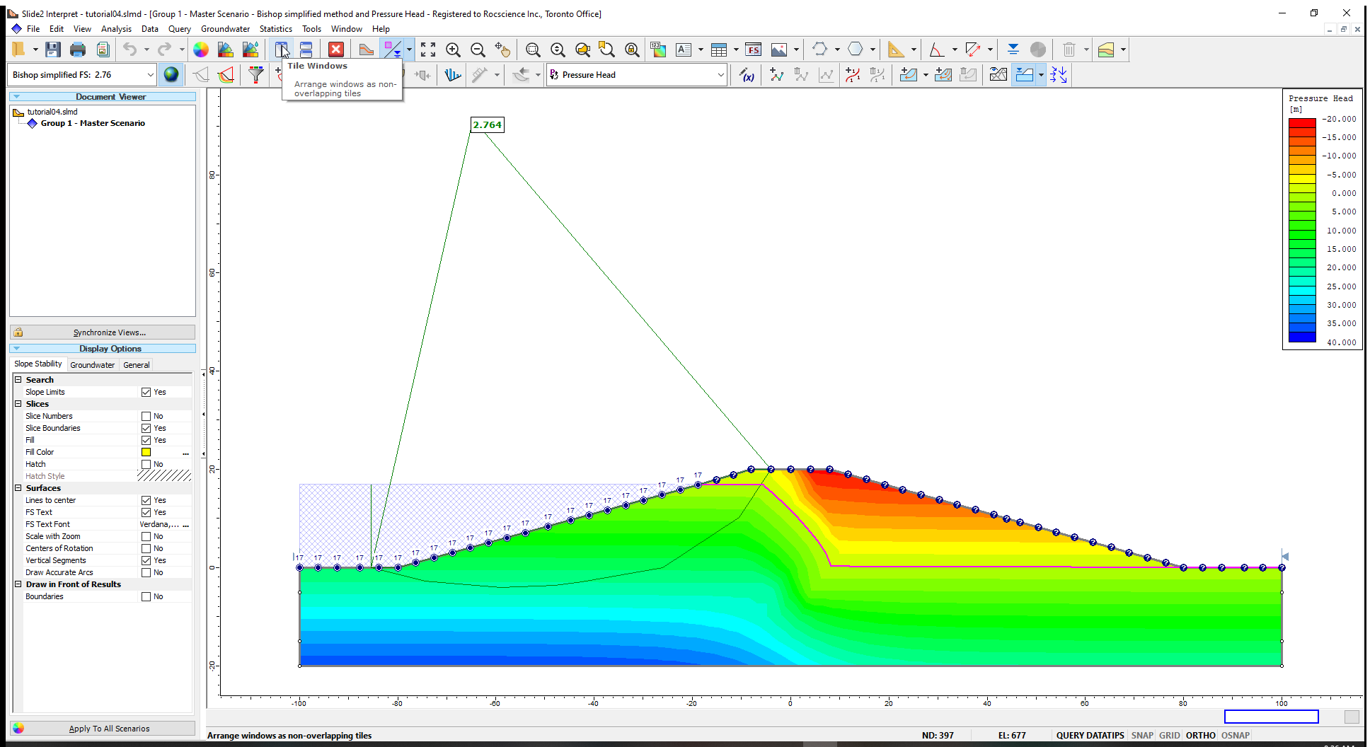
We can graph the pore pressures along the Global Minimum Slip Surface from the slope stability analysis.
- Right-click on the slip surface and select Add Query and Graph

- Select Pore Pressure and click Create Plot.
All graphs can be exported to Excel by clicking on the icon 
6.3 UNSATURATED SHEAR STRENGTH
The Unsaturated Shear Strength Angle is usually not a well-known quantity, which can increase factor of safety if the failure surface passes through unsaturated zones. To appreciate its importance, parametric studies, in which Unsaturated Shear Strength angle is varied between 0 and the Friction Angle of a material, can be conducted using the Sensitivity Analysis option in Slide2 (which will be covered in a later tutorial).
To try our hand at unsaturated strength analysis, we specify an Unsaturated Shear Strength Angle for the clay core and re-run the slope stability analysis. This is left as an additional exercise for the user.