5 - Transient Groundwater Analysis

1.0 Introduction

Steady-state seepage analysis, which was covered in Tutorial 4, is used to determine long-term or equilibrium groundwater (pore pressure) conditions that do not change with time.

In many cases, however, boundary conditions and pore pressures vary with time, and it can take a long time for seepage to reach steady state. Transient groundwater (seepage) analysis is used in such cases to determine time-dependent pore pressure changes and their effect on slope stability.

This tutorial will demonstrate a transient finite element groundwater analysis of an embankment dam in Slide2. We will analyze the following two scenarios:

Scenario 1: Changing pore pressures and phreatic surface in a dam due to rapid filling (represented by the application of a constant head boundary condition).

Scenario 2: Changing pore pressures and phreatic surface in a dam due to boundary condition changes over time.

In this tutorial we will learn to:

• Define the time stages at which we would like to observe pore pressures and the phreatic surface
• Define boundary conditions that vary over time (transient boundary conditions)
• Define a soil Water Content curve
• Run a slope stability analysis at any stage of a transient groundwater analysis
• Graph safety factors with time

The finished product of this tutorial can be found in Tutorial 05 Transient Groundwater Analysis. slmd from File > Recent Folders > Tutorials Folder.

2.0 Geometry

Begin by opening the tutorial starting file.

1. Select File > Recent Folders > Tutorials Folder.
2. Open Tutorial 05 Transient Groundwater Analysis - starting file.slmd.

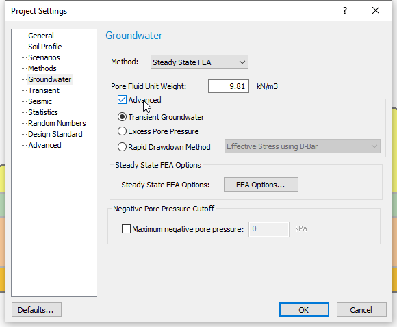
2.1 PROJECT SETTINGS

1. Select Analysis > Project Settings or click on the Project Settings icon to define the following parameters under the respective sections.
2. General tab:
• Stress units = Metric
• Time units = Months
• Permeability units = meters/second
3. Groundwater tab:
• Method = Steady State FEA

This method will be used as the initial state for the groundwater analysis. (You can also use the water surfaces or the grid pore pressure options).

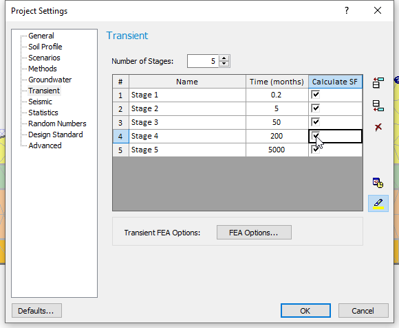
• Tick the Advanced checkbox and select the Transient Groundwater radio button.



4. Transient tab:

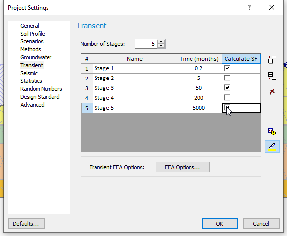
We will define five transient groundwater stages in which pore pressures will be observed.

• Enter Number of Stages = 5.
• Enter the parameters shown in the table below:

Name	Time (months)
Stage 1	0.2
Stage 2	5
Stage 3	50
Stage 4	200
Stage 5	5000



You can define the time using calendar dates by clicking on the Define by Date button on the right edge of the dialog. Times will be automatically calculated according to the specified dates.


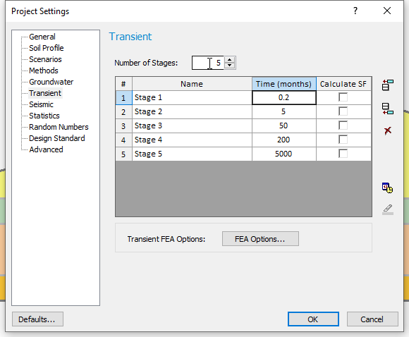
For this tutorial, we will view the seepage analysis results before computing the stability of the slope and we will therefore not select any of the Calculate SF checkboxes.

5. Click OK to close the Project Settings dialog. Steady State and Transient modes, in addition to the default Slope Stability mode, are immediately added to the application and appear as tabs below the model view.
6. Click on the Steady State Groundwater tab at the bottom of the model view.

2.2 DISCRETIZING AND MESHING

Before defining boundary conditions for finite element seepage analysis in Slide2, we must first discretize and create a mesh.

1. Select Mesh > Discretize and Mesh

We will use the default mesh in this model.

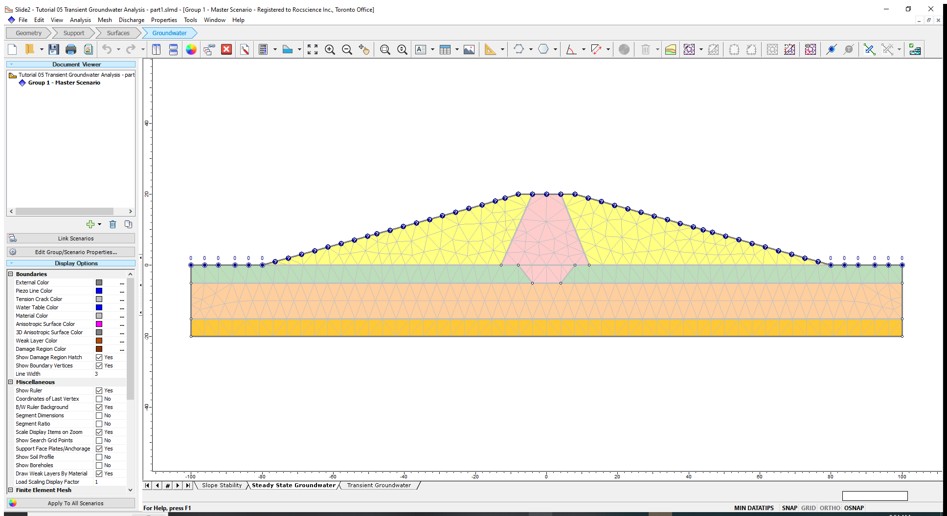
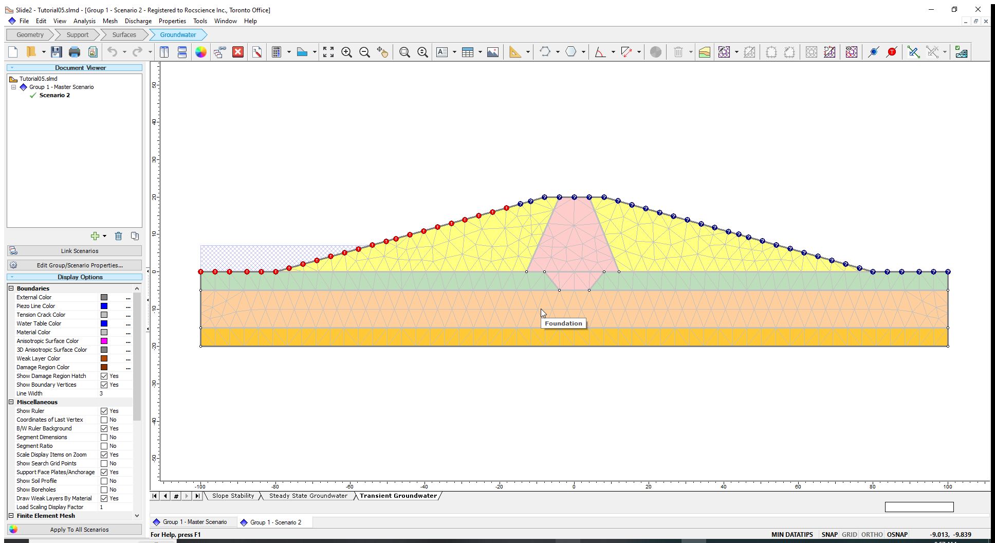
3.0 Boundary Conditions

We will now apply appropriate boundary conditions to the upstream and downstream faces of the model for both the initial steady-state and the subsequent transient phases of the model.

3.1 STEADY STATE GROUNDWATER BOUNDARY CONDITIONS

In the Steady State Groundwater tab, we will specify the starting steady state conditions (initial phreatic surface) for the embankment dam as being at the original ground level.

1. Select Mesh > Set Boundary Conditions or click on the Set Boundary Conditions icon .
2. Enter a Total Head Value of 0.



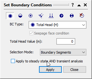
3. Select the horizontal segments of the ground surface on both the upstream and downstream sides of the dam.
4. Uncheck the box Apply to steady state AND transient analysis because we will be applying different boundary conditions.
5. Click Apply to assign the boundary condition as shown on the model below and close the dialog.

3.2 TRANSIENT GROUNDWATER BOUNDARY CONDITIONS

1. Select the Transient Groundwater tab at the bottom of the model view.

We will set up boundary conditions to simulate rapid filling of the dam on the upstream (left side) by applying a Total Head of 17 m to the upstream side of the model.

2. Select Mesh > Set Boundary Conditions or click on the Set Boundary Conditions icon .
3. Enter a Total Head Value of 17.



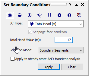
4. Uncheck the box Apply to steady state AND transient analysis, because we will be applying different boundary conditions.
5. Select the segments of the dam’s upstream (left side) and click on the Apply button to assign the boundary condition.
6. Close the dialog.

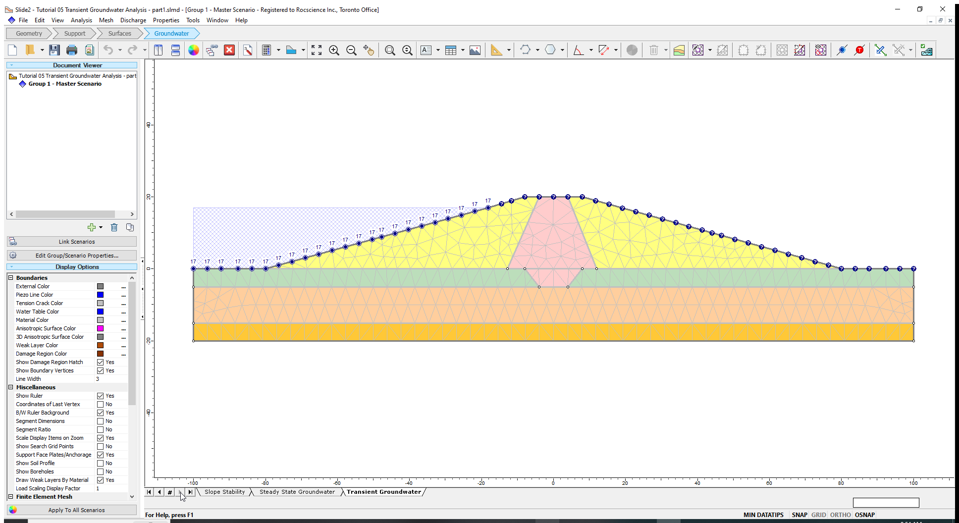
The Boundary conditions are now assigned to the model as shown below.

4.0 Hydraulic Properties

Both steady-state and transient groundwater analyses require the specification of hydraulic conductivities (permeabilities). Transient analysis additionally requires the specification of a water content curve.

In Slide2, the default permeability model assigned to materials is known as the “Simple” curve. It is also possible to define a custom permeability model (typically based on laboratory results). For this tutorial, we will define a custom permeability model and water content curve for the clay core and maintain the Simple curve for the other slope materials.

Check out the Define Hydraulic Properties help page for more information on the permeability models.

To define the water content curve for the clay core:

1. Select Properties > Define Hydraulic Properties or click on the Define Hydraulics Properties icon.
2. Select the Clay Core material and then click New.



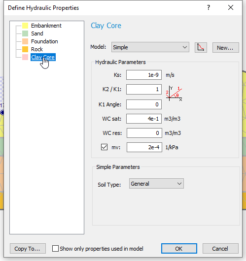
3. Enter Clay Core Curve as the name.
4. In the Permeability tab, enter the values below:

Point	Matric Suction (kPa)	Permeability (m/s)
1	0	1e-9
2	15	1e-9
3	50	1e-10
4	100	1e-11
5	200	1e-12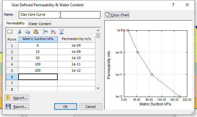



The curve indicates that permeability decreases with increasing matric suction.

5. Next, click on the Water Content tab and enter the values shown in the table below. This outlines a linear relationship in which water content drops as matric suction increases.

Point	Matric Suction (kPa)	Water Content
1	0	0.4
2	1250	0.1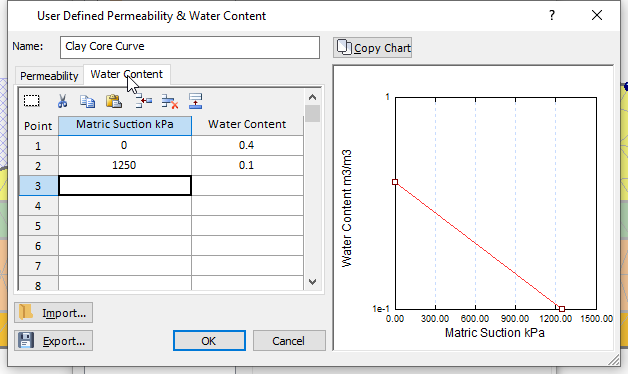



6. Click OK to close the data entry form and return to the Hydraulics properties dialog. Click OK to close this dialog as well.

We are now ready to compute the first scenario of our transient groundwater analysis.

5.0 Computation and Interpretation

1. Save the file and click on the Compute (Groundwater) icon.
2. Click OK to compute.

5.1 INTERPRETATION

1. Select Analysis > Interpret (groundwater) or click on the Interpret (Groundwater) icon in the toolbar to view results.

All five stages (defined in project settings) are computed and opened in different tabs in the Slide Interpret window.

2. By default, the initial stage is displayed. Select Pore Pressure from the contour data dropdown.

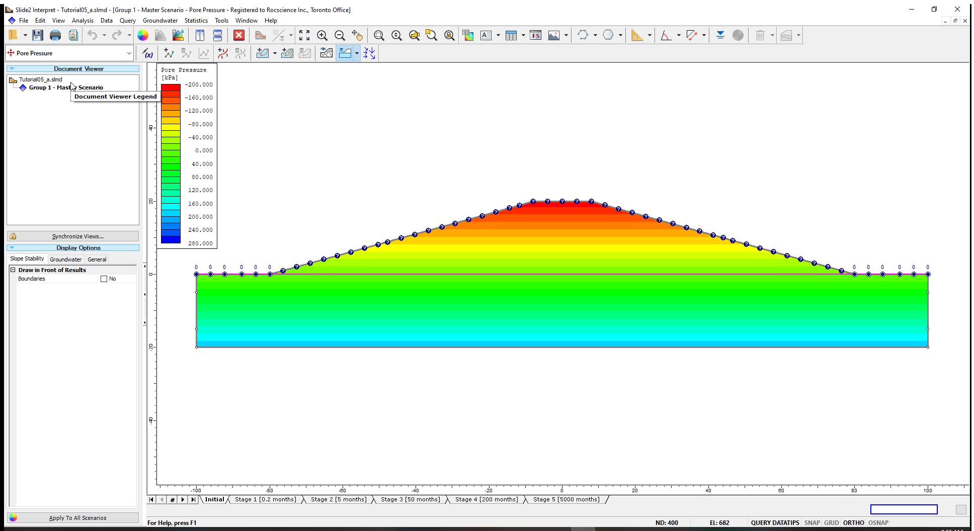
From the image above, the steady state phreatic surface is a horizontal line at zero elevation.

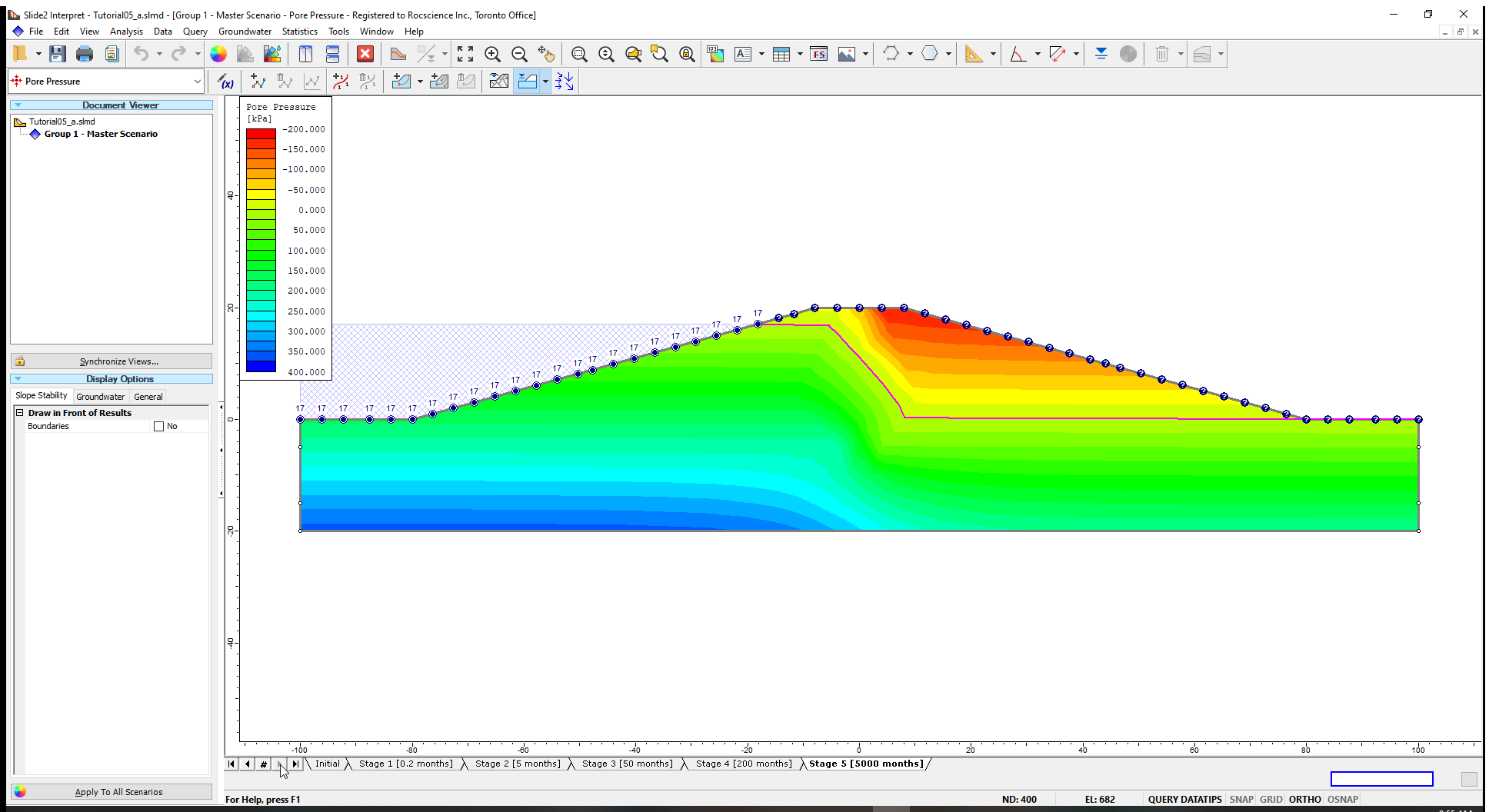
Cycle through the phreatic surface, pore pressure and head results for the different stages by clicking on the stage tabs. This will help us to view the pore pressure changes in the dam and the progression of the phreatic surface with time.

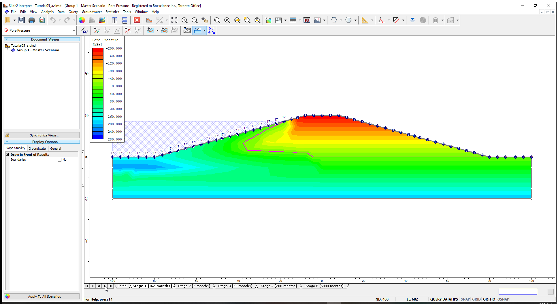
At Stage 1 (0.2 months) shown above, the wet phase resulting from the rapid rise in water level on the upstream face has not yet reached the core of the dam. The wet front progresses in the next stages until it reaches steady state/long-term conditions (when it no longer varies with time). The pore pressures at Stage 5(5000months) are at steady state.

You can also show the progression of the phreatic surface with time on a single model plot.

1. Select View > Display Options
   
2. Select the Groundwater tab and, under FEA water, select All Stages.
3. Click Done to see results.

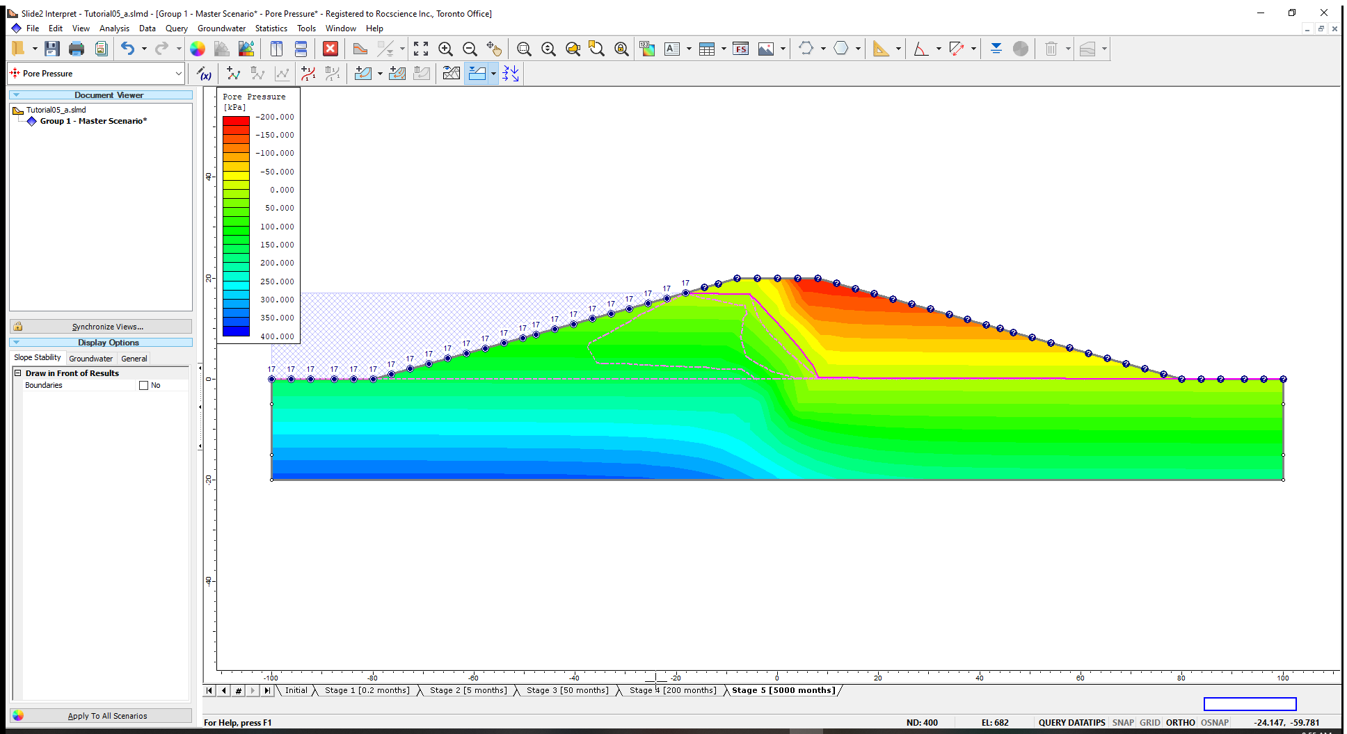
The solid pink line represents the water table (phreatic surface) at stage 5. The water tables at the other stages are plotted as light pink lines.

5.2 FLOW VECTORS

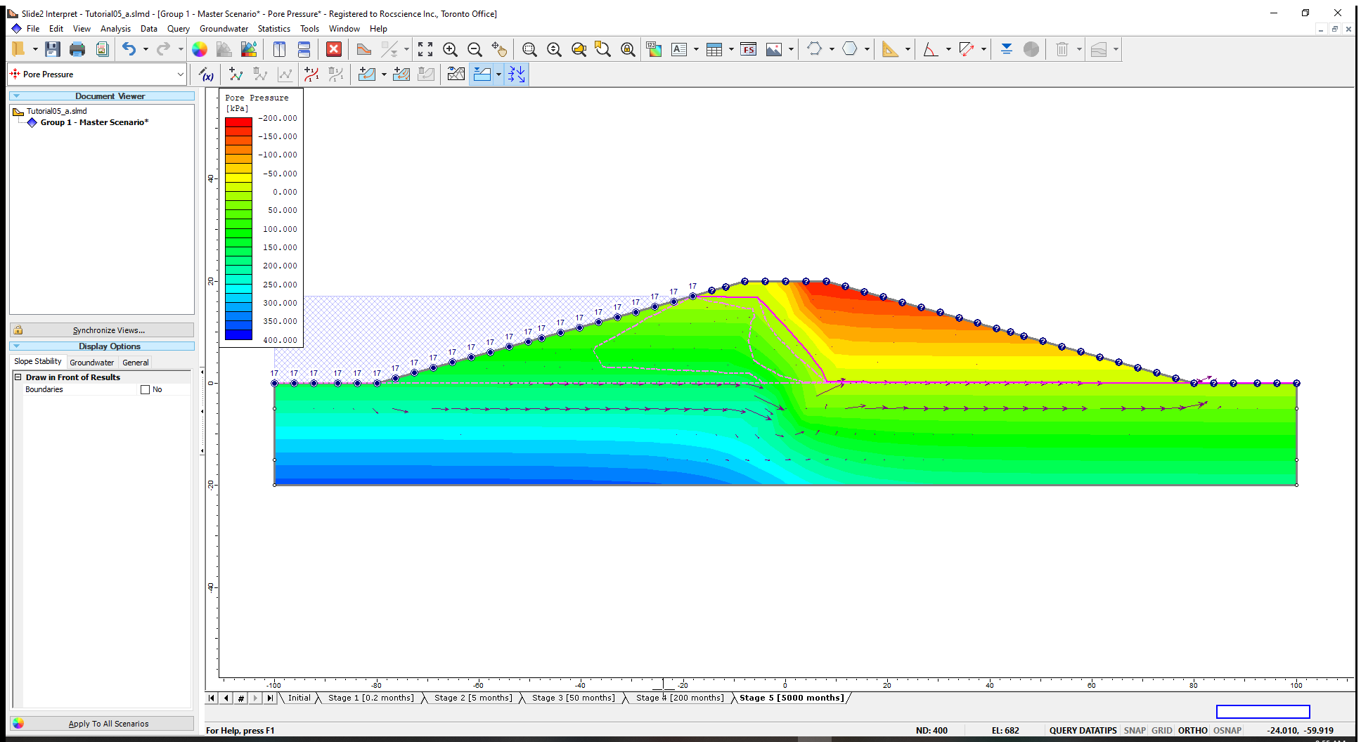
1. Click on the Flow Vectors icon in the toolbar to see the direction of groundwater flow.

The flow of water is towards the downstream side and aligns with the progression of the phreatic surface through the dam with time that we just saw from the stage tabs.

5.3 QUERY

We will query a single point (vertex) near the middle of the dam to view the change in pore pressure with time in detail.

1. Select Groundwater > Query > Add Material Query
   
2. Enter the coordinates (-3, 6) in the Command prompt and press the ENTER key twice to finish entering the coordinates of the point.



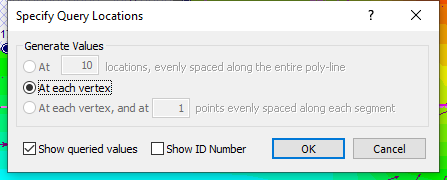
3. Click OK to close the dialog.

A plus sign (+), indicating the query point (you may need to turn off the flow vectors to see it), is shown on the model.

4. To graph the data, right-click on the (+) sign on the model and select Graph Data vs. Time.

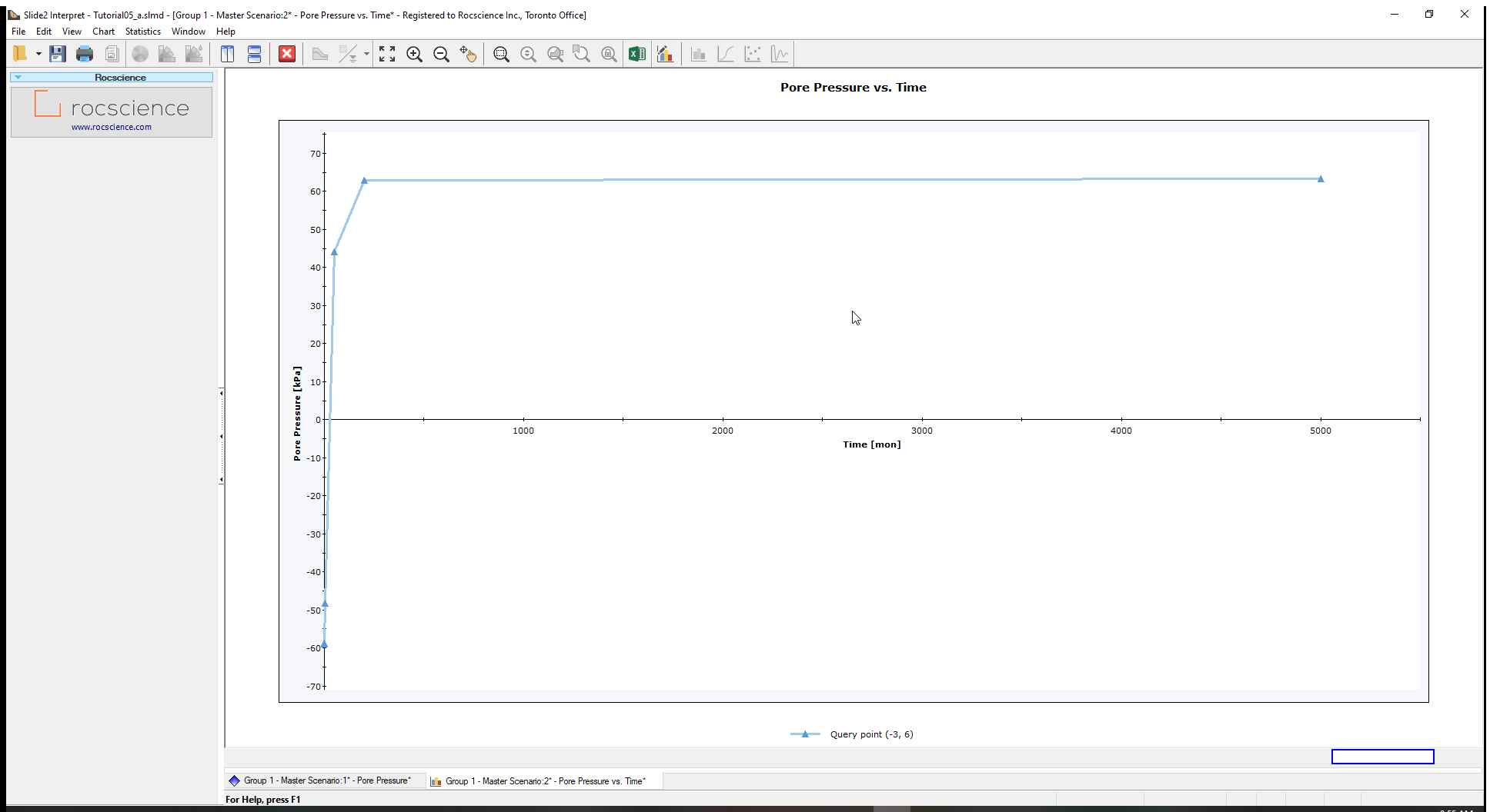
You will now see a plot of Pore Pressure with time at point (-3,6).

It is sometimes more informative to use a logarithmic scale for time. To change to this scale:

1. Select Chart > Chart Properties or click on the Chart Properties icon on the left sidebar.
2. Click Close.
3. Expand the Axes item and tick the checkbox for Logarithmic Horizontal Scale. Its status will change from ‘No’ to ‘Yes’.

The Logarithmic scale chart at point (-3,6) will be shown.

The chart shows that positive pressures do not reach the query location until about 15 months after rapid impoundment. Pore pressure reached its final (steady state) value at the location after about 200 months.

6.0 Slope Stability Analysis

After computing and interpreting our seepage analysis, we will now calculate safety factors for Stages 1, 3 and 5. (You can do it for all the stages if you so desire.)

To do this, use the following steps:

1. Close the chart with the red X button in the toolbar. Return to the modeller by selecting Analysis > Modeller
2. Select Analysis > Project Settings
   
3. Go to the Transient tab in the Project Settings dialog and tick the Calculate SF box for stages (1,3 and 5) as shown below. Click OK to close the dialog when done.
4. Click on the dropdown arrow beside the compute icon and select Compute (Slope Stability).



5. After the computations are done, select Interpret (Slope Stability) to view the results.

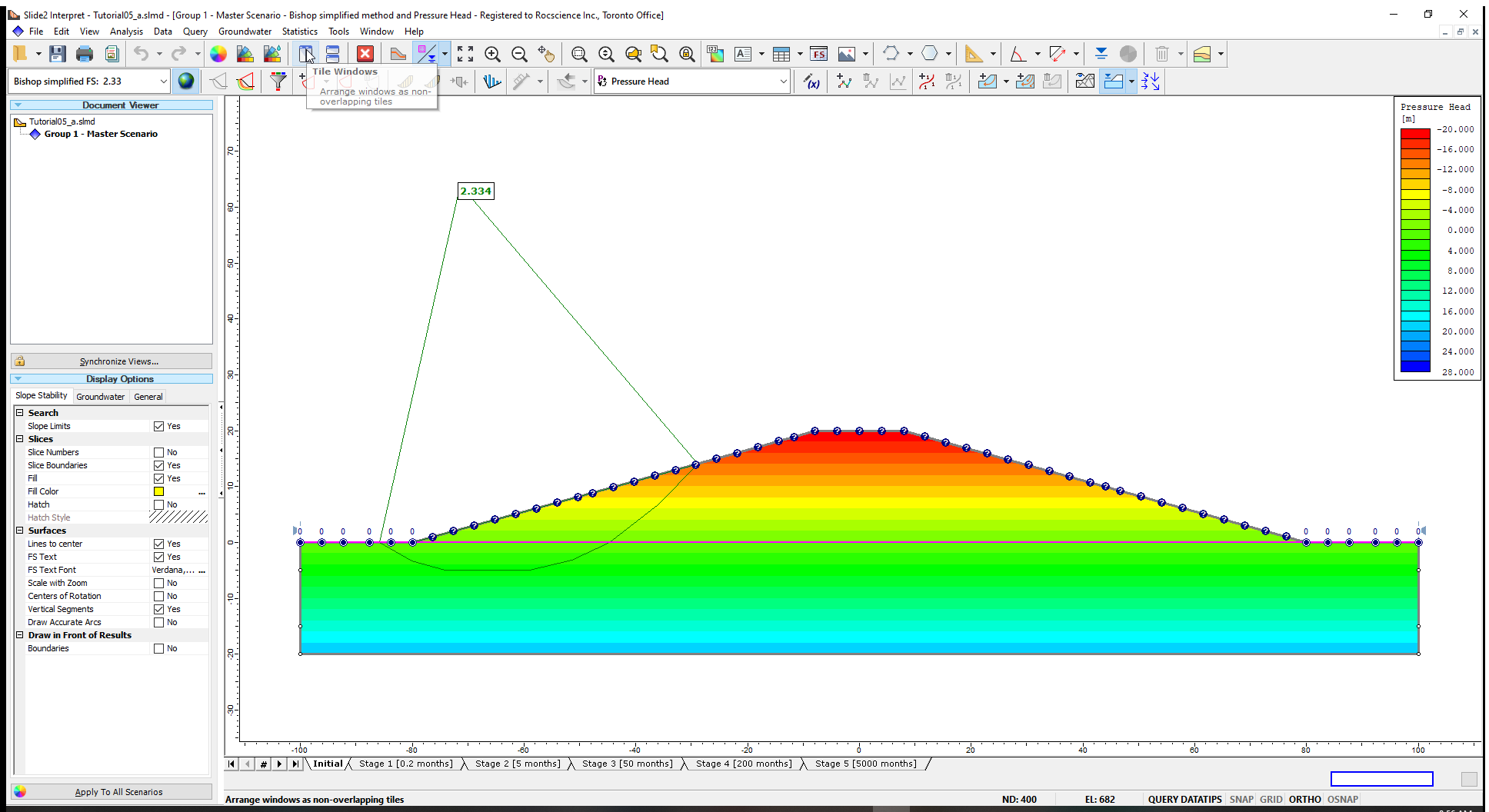
The safety factor at the initial state (prior to impoundment) is 2.3 as shown on the image above.

The factor of safety is highest at Stage 1 when the impounded water is first applied and reduces to 2.8 at Stage 3. It attains a steady state factor of safety value of 2.8 at Stage 5.

4. Close Interpret and return to the Modeller.

7.0 Transient Boundary Conditions (Second Scenario)

We will now model a second transient scenario in which boundary conditions vary with time.

1. Right-click on the Master scenario and select Add Scenario

In this scenario, we will define the transient boundary condition function that represents a gradual drawdown of the water level in the dam.

The function will specify Total Head values on the upstream that drop every 3 months.

To set up the boundary conditions:

2. Click the Steady State Groundwater (initial stage) tab at the bottom of the screen and set the boundary conditions to a Total Head of 17m for the upstream of the dam.



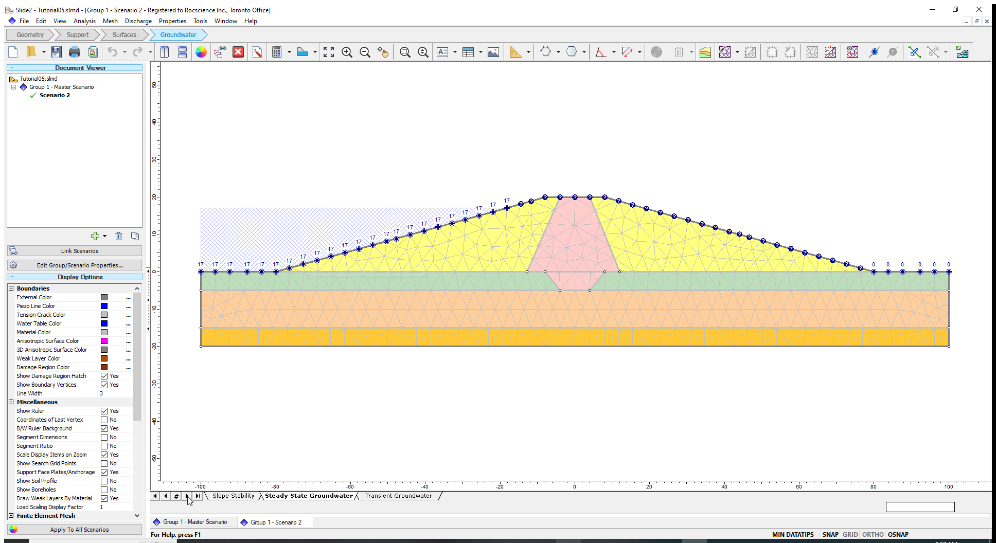
3. Click on the Transient Groundwater tab.
4. Select Mesh > Set Transient Boundary Conditions or click on the Set Transient Boundary Conditions icon.
5. Click the New button and enter Gradual Drawdown as the Function Name.
6. Enter the Time and Total Head values in the table below and click OK to close the dialog.

Time (month)	Total Head (m)
0	17
3	15
6	13
9	11
12	9
15	7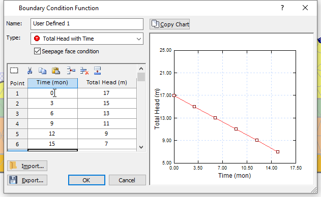



7. Click Close in the Set Transient Boundary Conditions dialog.
8. Right-click on the upstream boundary segments. Select Set Total Head (Gradual Drawdown) from the dialog and apply the transient conditions to the boundary.

A view of the model with the Total Head value at the end of the simulated period will be displayed (see the figure below).

In this scenario, we will calculate the safety factor for all the stages.

7.1 Computation and Interpretation

Save the model and compute both the groundwater and slope stability components.

1. Click on the dropdown arrow beside the Compute icon and select Compute (slope stability).
2. Scenario 2 will be automatically selected since it does not yet have results. Click OK.

To view the results:

3. Click on the dropdown arrow beside the Interpret (groundwater) icon and select Interpret (Slope Stability).

Click through the stages using the tabs at the bottom and observe the pore pressure variations as the impoundment levels are lowered.

As the water table is lowered, the factor of safety decreases because of the reduction in the weight of the water.

8.0 Additional Exercise: Graph SF with Time

1. Return to the Modeller and in Project Settings > Transient, check the Calculate SF box for all stages:

Recompute the file and view the results. Let’s see the change in FS with time.

2. Select Data > Graph SF with Time.
3. Check the Spencer and GLE/Morgenstern-Price boxes.
4. Click Plot to see both graphs

You can clearly see the rapid decrease in factor of safety as the water table is lowered and the gradual increase as the initial excess pore pressures dissipate.

This concludes the tutorial.