1 - Quick Start Tutorial

1.0 Introduction

This quick start tutorial will demonstrate some basic features of Slide2. It will introduce the beginner to steps for building and computing models and analyzing results in Slide2.

This tutorial will analyze the stability of a simple, homogeneous slope by computing the critical factor of safety and the corresponding circular-shaped slip surface.

At the end of this tutorial, you will:

• Be able to build a simple model
• Compute the model, view, and interpret results, and
• Incorporate images from the analysis in an automatically generated Slide2 report

All Slide2 tutorial files are installed with the program and can be accessed by selecting File > Recent > Tutorials from the Slide2 main menu. You can find the finished product of this tutorial in the file Tutorial 01 QuickStart.slmd.

2.0 Getting Started

Open Slide2 on your computer. When the software is successfully launched, a new blank document will open, and your screen should look like the image below:

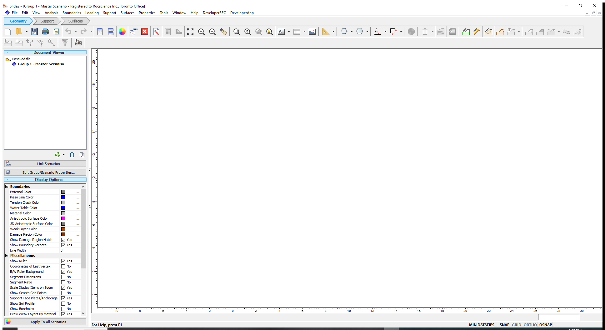
The program's Menu bar, which allows users to access all the program features, is located at the top of the screen. The Workflow tabs, which groups quick access icons or shortcuts, are directly below the menu bar. The program's Toolbar directly follows below the Workflow tabs. The Document Viewer and Display options are in the sidebar on the left.

Immediately beneath the model viewing window, at the bottom right corner of the interface, is the Command box (Prompt line). Below the Command box are DATATIPS, GRID, and SNAP options.

You can obtain assistance on Slide2 features using the Help option in the menu. It provides links to tutorials, theories, and documents. You can also click on the ‘?’ icon in the top right corner of any dialog to view the Help article for that specific feature.

3.0 Project Settings

The main parameters that control important analysis aspects in Slide2 are defined under Project Settings. These parameters include scenario options (whether the model will use only a single scenario or consider multiple sub-models), methods of slices selection, groundwater analysis type and choice of deterministic or statistical analysis.

To set our parameters for this tutorial:

1. Select Analysis > Project Settings from the menu or click on the Project Settings icon in the toolbar. The project settings dialog will open.
2. Under the General tab, we will retain the default options for Units of Measurement, Failure Direction and Data Output.



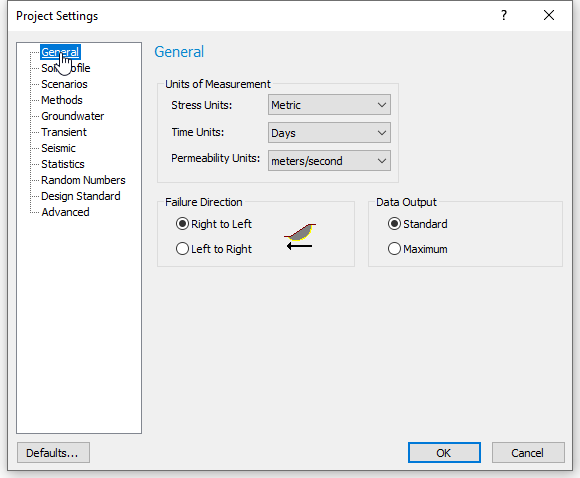The default for Data Output (Standard) only saves detailed results for the Global Minimum Slip Surface to minimize file size. (The Maximum option, on the other hand, saves information for every slip surface analyzed and can create huge files.)
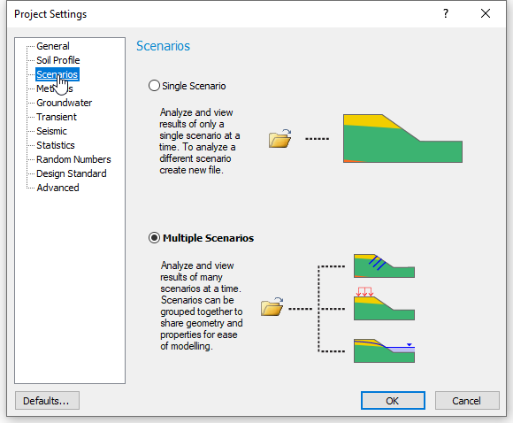
3. Next, select the Scenarios tab.
4. Although we will not create multiple scenarios, we will maintain the default Multiple Scenarios option.

The Multiple Scenarios option allows you to analyze several sub-models which use different model options and parameters such as slope angle, search methods, slope limits and groundwater conditions.



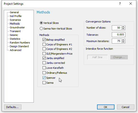
5. Finally, select the Methods tab.
6. We will retain the default ‘Vertical Slices’ option. (We will treat the Sarma non-vertical slices in a different tutorial.)

The Bishop Simplified and Janbu Simplified are the default analysis methods in Slide2. For this tutorial, we will use the Spencer method in addition to the defaults. To do so:

7. Under Methods, select the checkbox for Spencer analysis method.
Safety factors are calculated only for the methods chosen when we compute models. Click here to see more information on the different methods of analysis available in Slide2.

8. We will also retain the default options under the Convergence Options.
9. Click OK to close the dialog.

4.0 Project Summary

Before creating the model, let us give the project a title.

1. Select Analysis > Project Summary in the menu. A dialog will open.



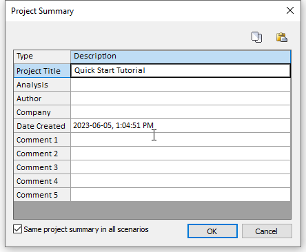
2. In the Project Title field, enter ‘Quick Start Tutorial’ (as seen above).
3. Click OK to close the dialog.

At this point, you should save your work. To do so, go to File > Save As and save as 'Quick Start Tutorial.'

5.0 Model

After defining the primary Project Settings, we can now create the model.

5.1 EXTERNAL BOUNDARY

As a first step, we must define our External Boundary, the overall geometry of the slope, that we will analyze in this tutorial. Our External Boundary will have the following coordinates:

(0,0); (130,0); (130,50); (80,50); (50,30); (0,30)

To enter the coordinates:

1. Select Boundaries > Add External Boundary in the menu or click the Add External Boundary icon in the toolbar.
2. The Prompt (Command) line is activated.

There are various methods of entering x and y coordinate pairs in Slide2. For this tutorial, we will use the coordinate table option.

3. Enter 't' in the command line and press the ENTER key.



4. The coordinate table will appear. Enter the coordinates in the table as shown below.



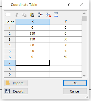
X	Y
0	0
130	0
130	50
80	50
50	30
0	30

5. Click OK to close the dialog.

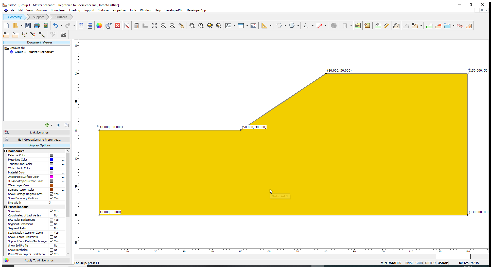
Slide2 displays the external boundary based on the coordinates entered.

6. Enter the letter ‘c’ in the prompt line to close the external boundary and exit the Add External Boundary mode.

Your model should look like the image below.

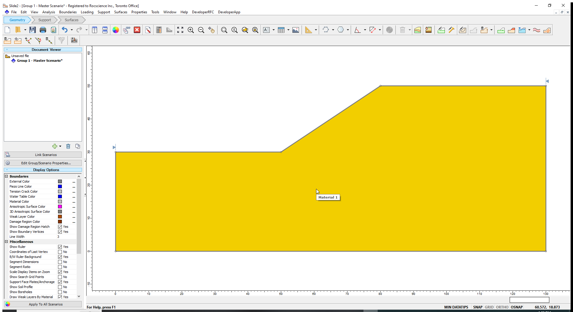
The area enclosed by the boundary is assigned the first default material defined under Material Properties, discussed in subsection 4.3. To learn about the other methods of entering coordinates, please refer to the Entering Coordinates help topic.

REMINDER: Do not forget to save your work regularly as you model. At least, save after every step that involves several actions (such as entering multiple coordinate pairs).

While it is not a critical modelling step, we will view the coordinates of the External Boundary.

1. Select View > Show Coordinates
2. Select the checkbox for External Boundary, as shown in the dialog below.
3. Click Close when you are done.

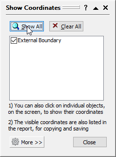
The coordinates for the External Boundary will now be displayed on the model.

5.2 SLOPE LIMITS

Once an External Boundary has been created in Slide2, the software automatically sets slope limits (the region along the slope surface within which the leftmost and rightmost points of slip surfaces must lie). The Slope Limits are displayed with two triangular markers at the left and right edges of the upper surface of the External Boundary.

You can modify the slope limits locations or specify two sets of limits. We will explore these options in other tutorials.

This tutorial will maintain the slope limits automatically set by Slide2.

5.3 MATERIAL PROPERTIES

We shall now specify the properties of the slope material.

1. Select Properties > Define Materials from the menu or click on the Define Materials icon in the toolbar.

You can also quickly access the Material Properties dialog by double-clicking anywhere on a material in a slope region.

2. In the resulting dialog, select Material 1 from the list on the left and enter the parameter values shown in the table below:

Name	Soil 1
Unit Weight	19
Strength Type	Mohr-Coulomb
Cohesion	5
Phi	30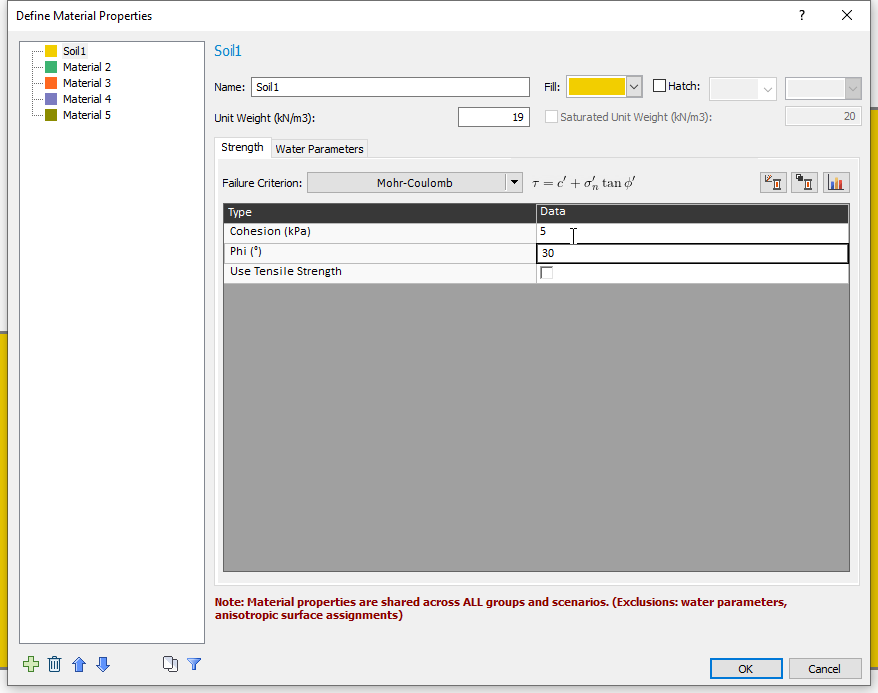



3. Click OK to close the dialog.

5.4 CRITICAL SLIP SURFACE

By default, Slide2 assumes failure surfaces to be Circular and applies the Auto Refine Search method to find critical slip surfaces. We will retain this default method for the current tutorial. (We will use the non-circular surface type and other search methods in our next tutorial).

1. Select Surfaces > Surface Options from the menu or select the Surfaces workflow tab and click on the Surface Options icon in the toolbar. This action will open the following dialog:
   
   
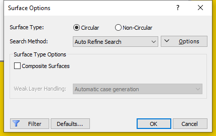
2. We will not change the default options.
3. Click OK to close the dialog. The model is complete, and we are now ready to compute it.

Refer to the *Search Methods help page for more information on Slide2 search methods.

6.0 Compute

1. Select Analysis > Compute from the menu or click on the Compute icon in the toolbar.

The Slide2 Compute engine will start up and run the simulations. This simple model will only take a few seconds to compute.

The Compute engine will close and disappear from the screen when calculations are completed. You are now ready to view the results.

7.0 Results

To view the analysis results:

1. Select Analysis > Interpret from the menu or click on the Interpret icon in the toolbar.

The results will open in a new window called the Interpreter (or Slide2Interpret).

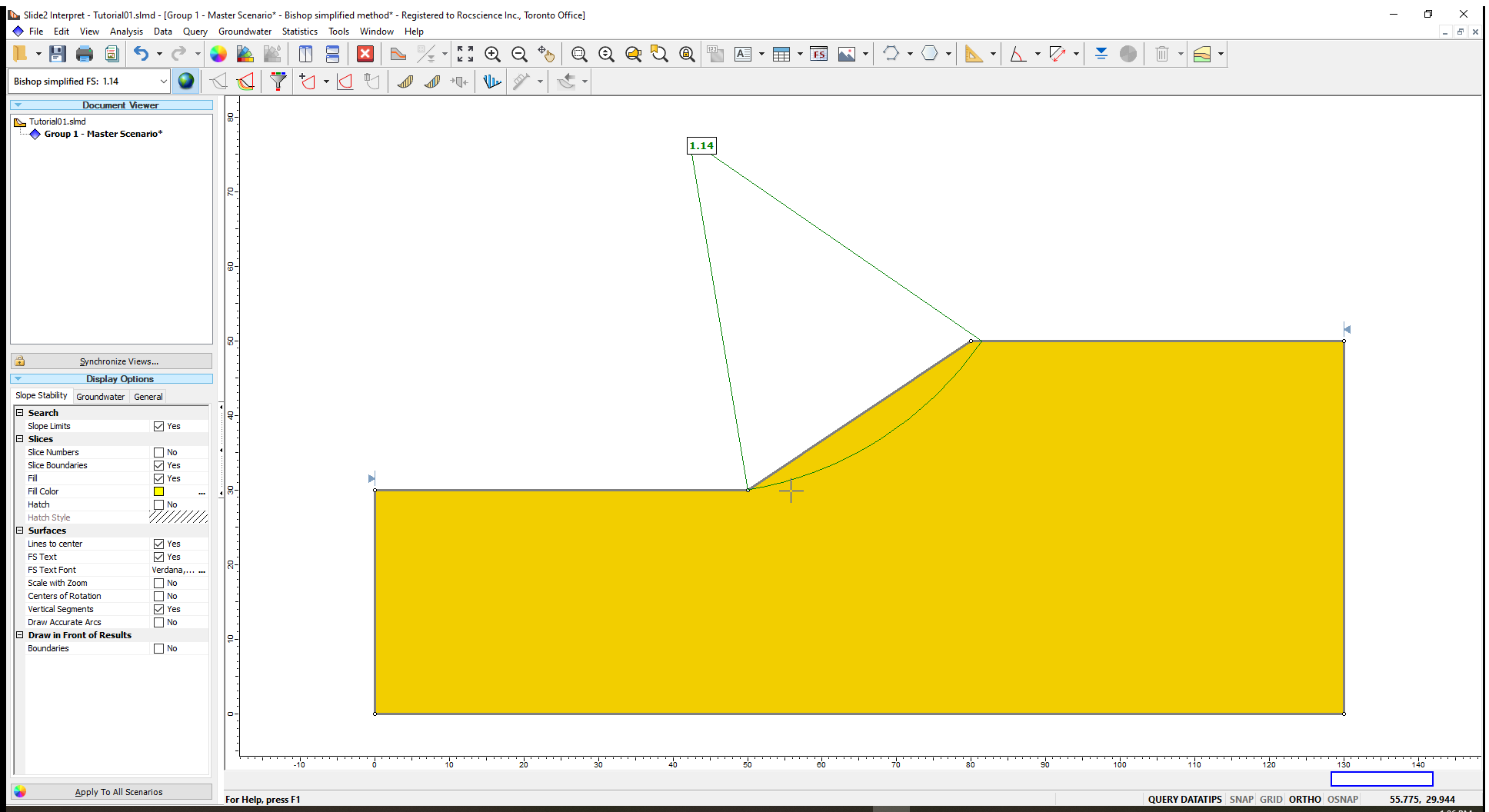
The primary outcomes of a Slide2 analysis are the lowest factors of safety, calculated according to the selected methods of slices (in our case, these were the Bishop Simplified, Janbu Simplified and Spencer methods), and the corresponding slip surfaces. The factors of safety and critical slip surfaces (Global Minimum Surfaces) are shown in the View window of Slide2Interpret.

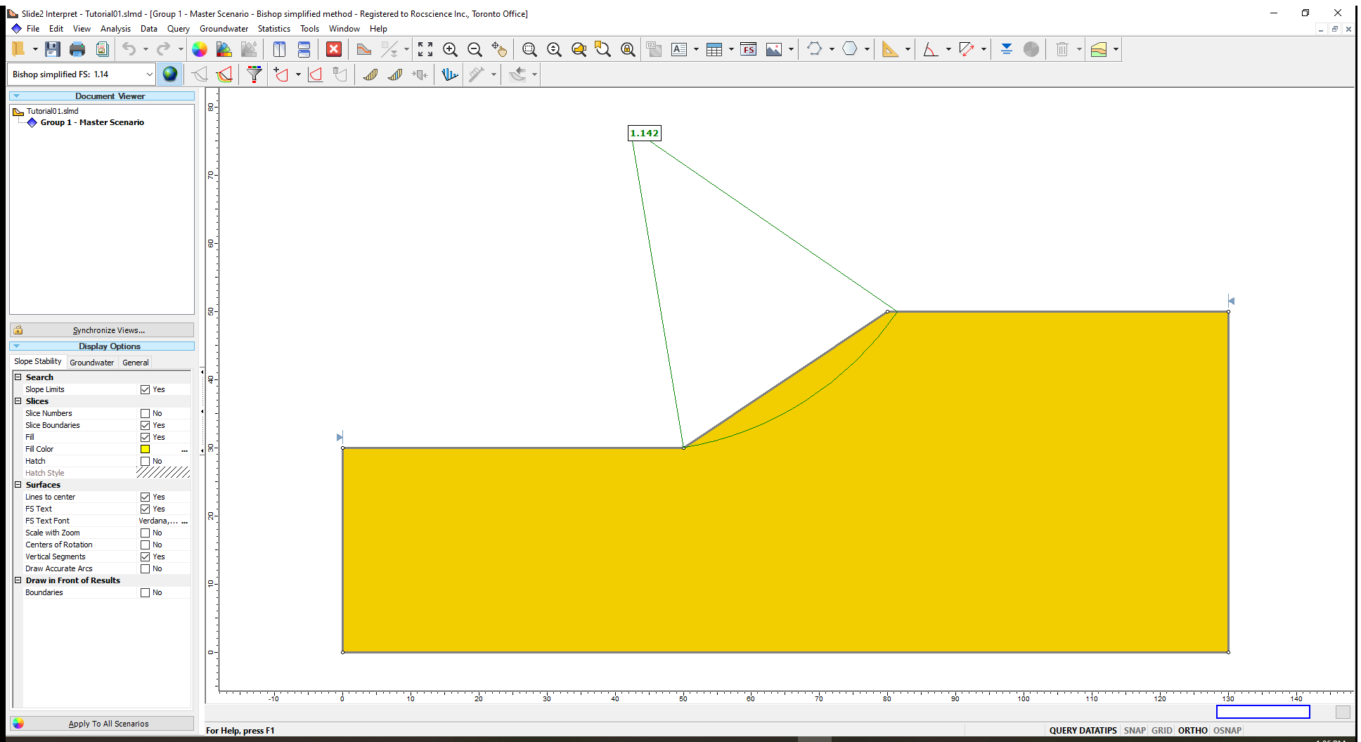
The reported Bishop Simplified factor of safety is 1.142. By default, safety factors are displayed with three decimal places. We can edit the number of decimal places.

To reduce the number of decimal places to two:

1. Select View > Legend Options from the menu bar of the Slide2Interpret window.
2. Change the number of decimal places to 2 in the ensuing dialog.
   
   
   
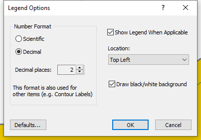
3. Select OK to close the dialog.

The safety factor for the critical slip surface is now shown in two decimal places on the model.

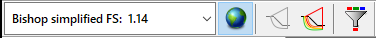
You can view the safety factors for the other analysis methods we specified in Project Settings by simply selecting the drop-down menu in the analysis method display box (shown below).

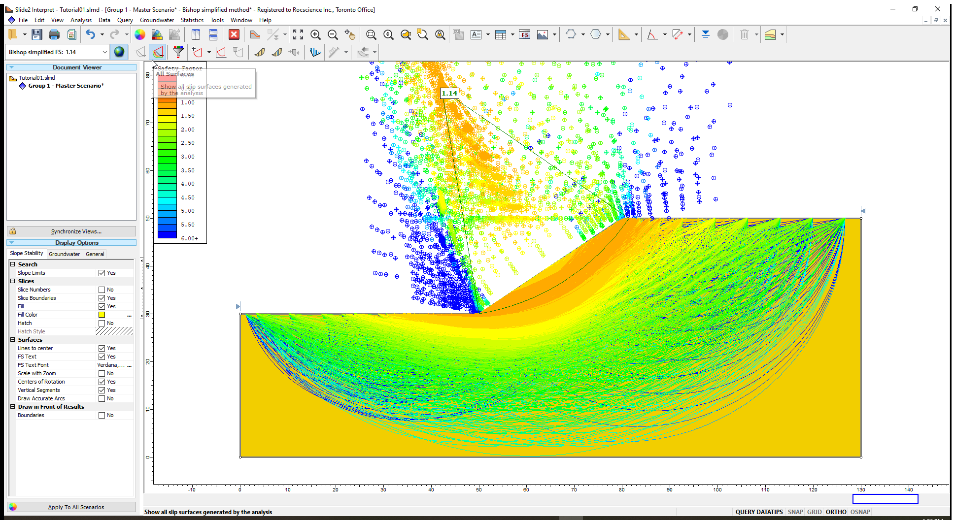
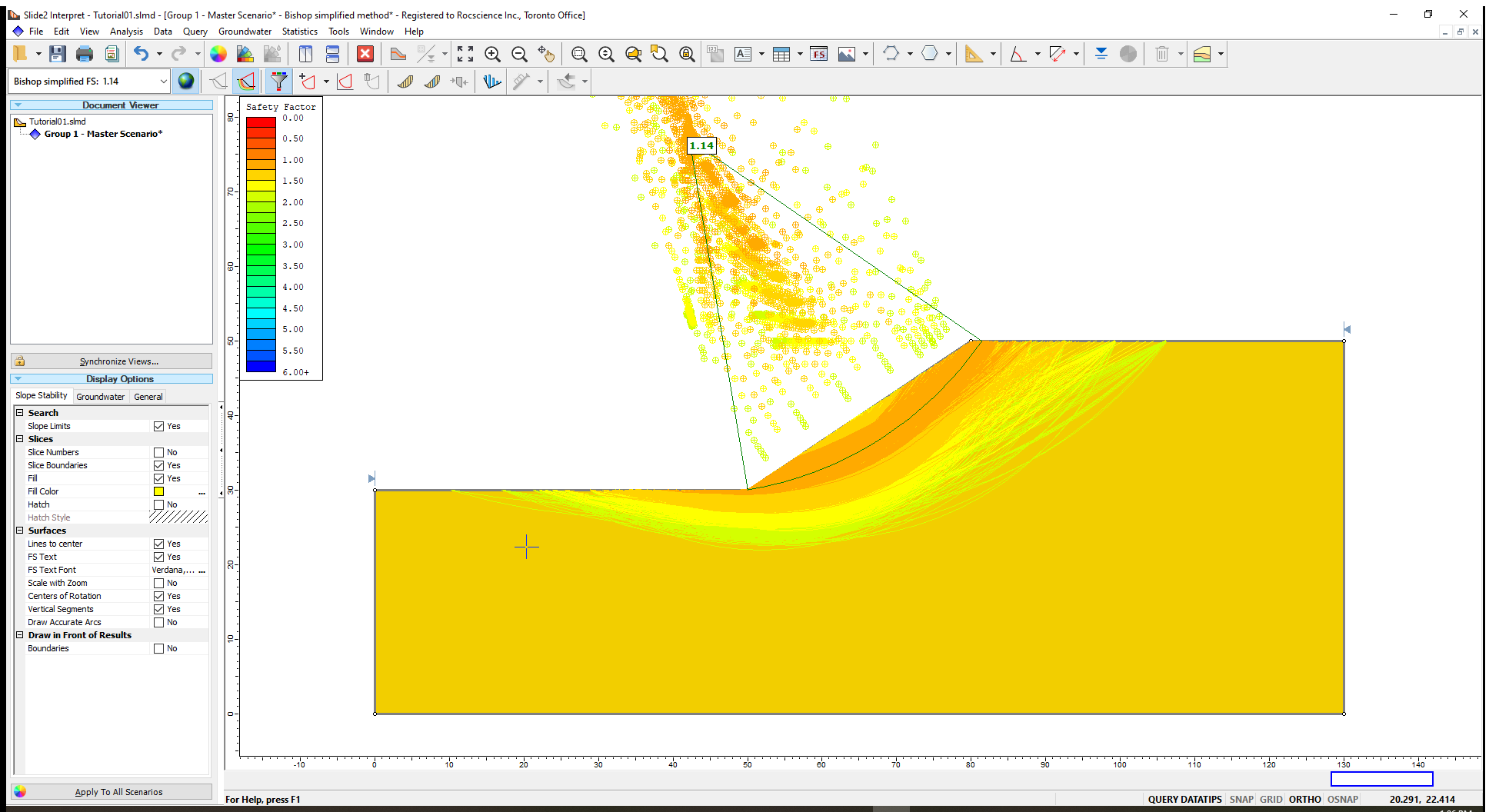
To view all the valid slip surfaces generated by the analysis:

1. Select Data > All Surfaces from the menu bar or click the All Surfaces icon in the toolbar.

All the slip surfaces analyzed for the Bishop Simplified method are displayed.

You can view all slip surfaces for the Janbu Simplified and Spencer methods by changing the analysis method in the drop-down menu.

The Contour Legend at the top left of the model view describes the factor of safety ranges with different colours and applies the colours to the corresponding slip surfaces.

In Slide2, you can filter slip surfaces according to various criteria. This tutorial will filter and display only slip surfaces with safety factors below 2 for the Bishop Method.

To filter the surfaces:

1. Select Data > Filter Surfaces in the menu or click on the Filter Surfaces icon in the Toolbar.

The following dialog will open:




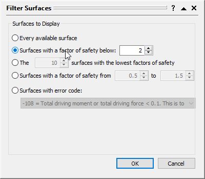
2. Select the second option, 'Surfaces with a factor of safety below.'
3. Set the threshold value as 2.
4. Click OK to close the dialog.

This action leads to only the filtered surfaces being displayed in the View window.

You can view filtered results for the other methods using the above-outlined approach.

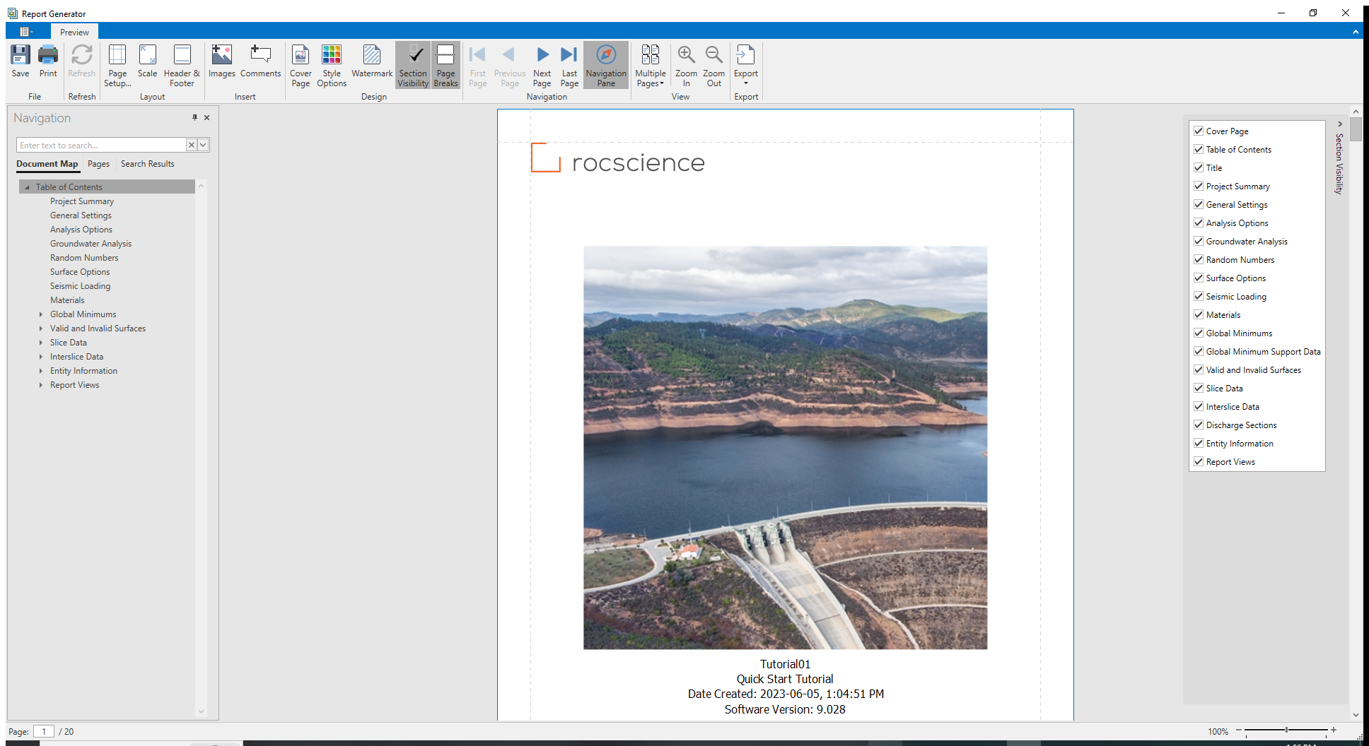
8.0 Report Generator

Slide2's Report Generator summarizes model input information, analysis options used, results of the analysis and other essential modelling information for the project.

You can add images of your model results in Slide2 Interpret to your generated report.

1. Select View > Add View to Report in the menu.
2. In the ensuing dialog, you may set a name for the image to be added to your report.
   
   
   
   
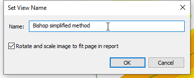
3. Click OK to close the dialog. The image will be added to your report.

To generate the report for your work:

4. Select Analysis > Report Generator in the menu or click on the Report Generator icon. (You can also activate the Report Generator from the Slide2 Modeller unit.)

This action will generate the report for this tutorial.

You can scroll through it to view summaries of the different parts of the model.

We have come to the end of our Slide2 quick start tutorial.