17 - Generalized Anisotropic Material

1.0 Introduction

This tutorial describes how to simulate an anisotropic material in Slide2. There are multiple ways of doing this, but the emphasis of this tutorial will be on using the Generalized Anisotropic option, which allows you to specify different material types in different directions.

At the end of the tutorial, we will know how to

1. Incorporate anisotropic behaviour into a model;
2. Use anisotropic surfaces.

The finished product of this tutorial can be found in the Tutorial 17 Generalized Anisotropic.slmd data file. All tutorial files installed with Slide2 can be accessed by selecting File > Recent Folders > Tutorials Folder from the Slide2 main menu.

2.0 Model

For this tutorial, we will read in a file.

1. Select File > Recent Folders > Tutorials Folder from the Slide2 main menu and open Tutorial 17 Generalized Anisotropic – starting file.slmd.

2.1 MATERIAL PROPERTIES

For the slope material, we will use the Generalized Anisotropic option. This allows you to specify different material types in different directions. Before we set up the Generalized Anisotropic material, let’s look at the sub-materials that make up the generalized material. For this example, we will assume the soil has weak, subhorizontal bedding. Two materials have been set up: one that represents the direction parallel to bedding (called Bedding) and one that represents all other orientations (called Soil Mass).

1. Select Properties > Define Materials from the menu.
2. Look at the Soil Mass and Bedding materials. These two materials will be assigned to a Generalized Anisotropic material as described below.
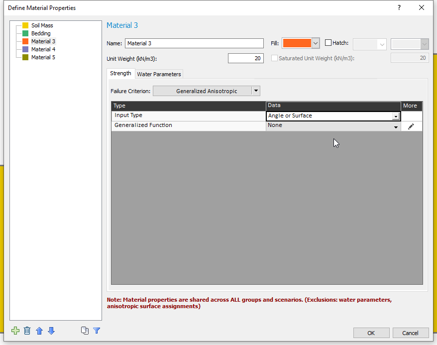
   In this case, both sub-materials use Mohr-Coulomb strength but have different values of cohesion and friction angle. However, any strength type can be used as a joint or base for a Generalized Anisotropic material. Take note that Soil Mass has cohesion of 5 while Bedding has cohesion of 0. We will refer to this in the results section.
3. Click on Material 3. Change the Strength Type to Generalized Anisotropic.
   Notice the Input Type dropdown which contains the options “Angle range” and “Angle or surface.” The “Angle range” option is a legacy option. All of its functionality can also be done in the newer and more flexible “Angle or surface” option.
   
4. Set the Input Type to Angle or surface.
   
5. Click the pencil icon next to the Generalized Function input.
   You will see a dialog in which you can specify different materials over different angular ranges. We want the Bedding material to be active within plus/minus 10° of horizontal and the Soil Mass to be active in all other directions. However, within the 5° range between the weak region and the rest, we want to interpolate the strengths of the joint and base materials. Angles in the dialog are measured from the +x direction, so 90° represents vertical.
   
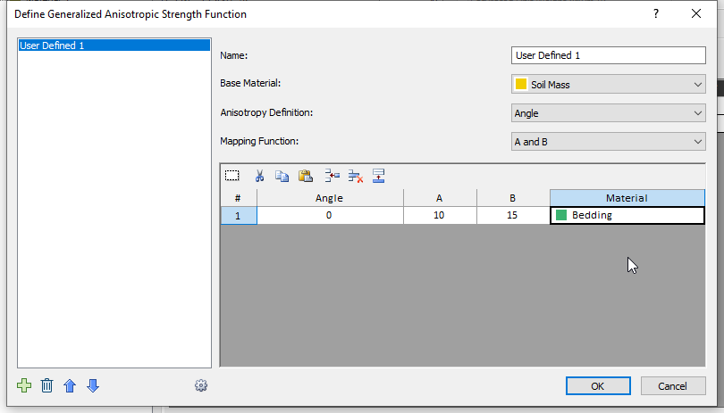
6. First, change the name to “Angle Function.”
7. Set the Base Material to Soil Mass.
8. Since we want stepwise change in strength with some interpolation, we will use the default “A and B” Mapping Function. You can also interpolate the strengths through the entire range using Linear or Cosine. More information can be found on the Generalized Anisotropic help page.
9. Enter:
• Angle = 0
• A = 10
• B = 15
• Material = Bedding.

As already stated, this means that if the angle of the base of the slice is between -10 and 10 (-A, +A), the strength of the Bedding material will be used. If it is between -15 and -10 (-B, -A) or between 10 and 15 (A, B), the strengths of the Bedding and Soil Mass materials will be interpolated. And outside of this range, i.e., greater than 15 (B) or less than -15 (-B), the strength of the Soil Mass will be used.




10. Click OK.
    Material 3 is now assigned the Generalized Function ‘Angle Function’.
11. The material is currently named “Material 3.” Rename it to “Anisotropic Angle.”
12. Click OK to close the Define Material Properties Dialog.

2.2 ASSIGN MATERIALS

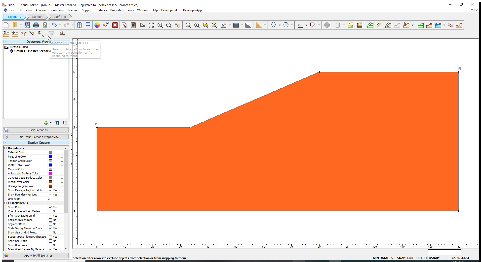
By default, the slope is assigned Material 1 (Soil Mass). We need to set the slope material to the Anisotropic Angle material that you defined above.

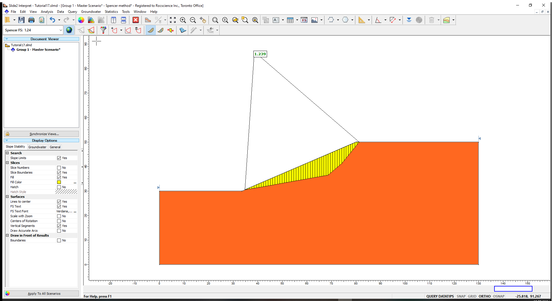
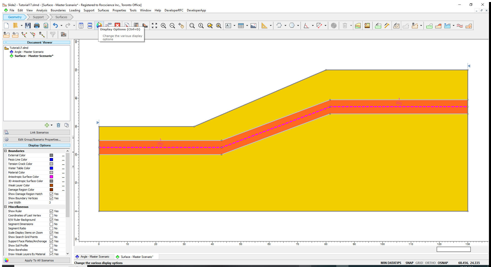
1. Right-click inside the model and select Assign Material > Anisotropic Angle. The model will look like this.

3.0 Compute

1. Save the model by selecting File > Save As in the menu.
2. Select Analysis > Compute in the menu to perform the analysis.
3. Then select Analysis > Interpret to view the results.

4.0 Interpret

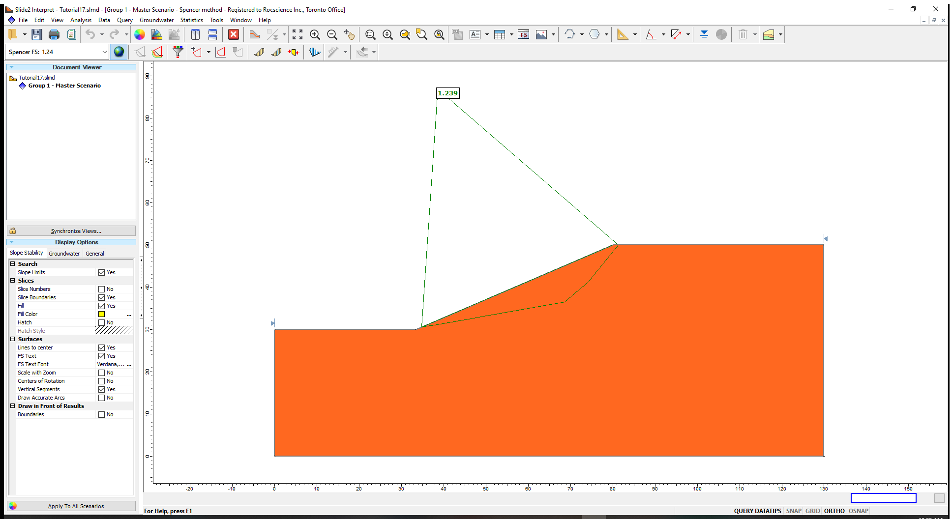
The Interpret program shows the results of the Janbu analysis (FS 1.182).

With the Generalized Anisotropic material model, the angle of the base of each slice determines which material is used to calculate the strength.

1. Go to Query > Show Slices
2. Click on a slice about halfway down the slope.
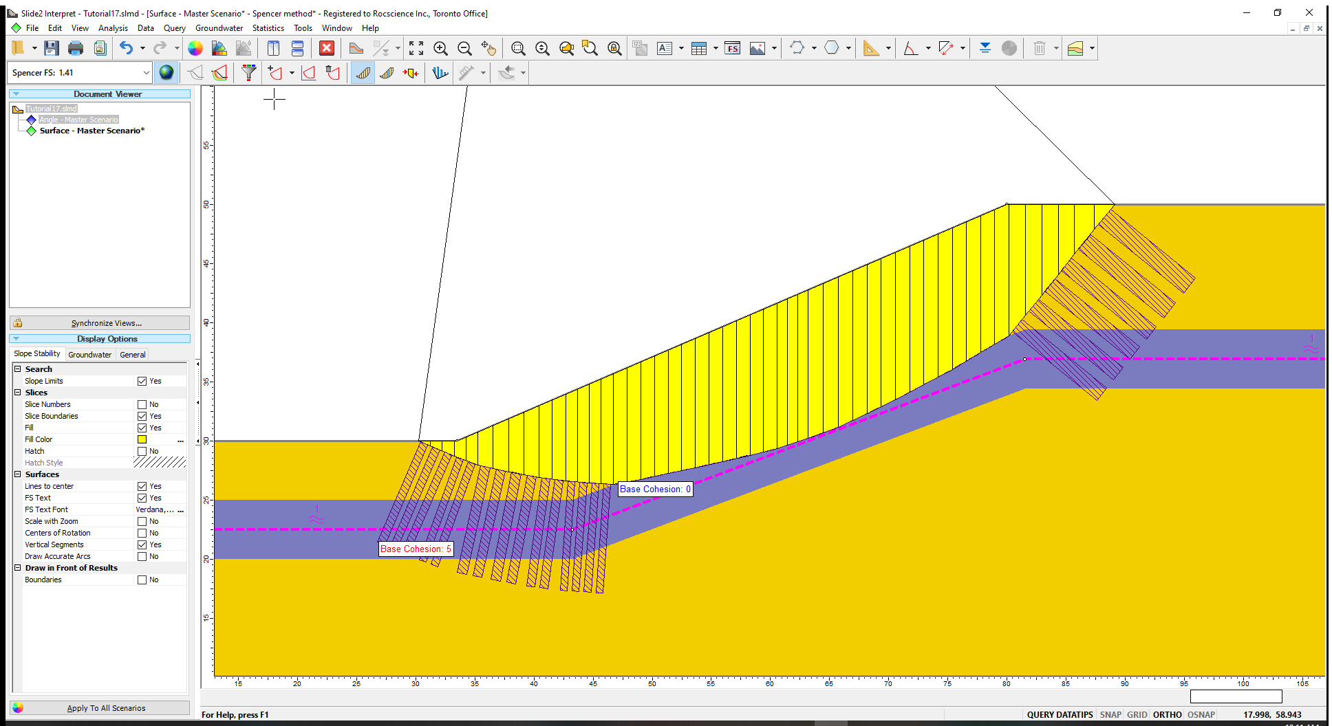
3. Select Query > Show Values Along Surface and set the Slice Data to Base Cohesion.
4. Click Done.
5. Notice that the base cohesion changes from 0 to 5. If you were to measure the angle of the left part using the Tools menu, you would be able to see that the angle is in the (Angle-A, Angle+A) range, and hence the Bedding material strength is taken.

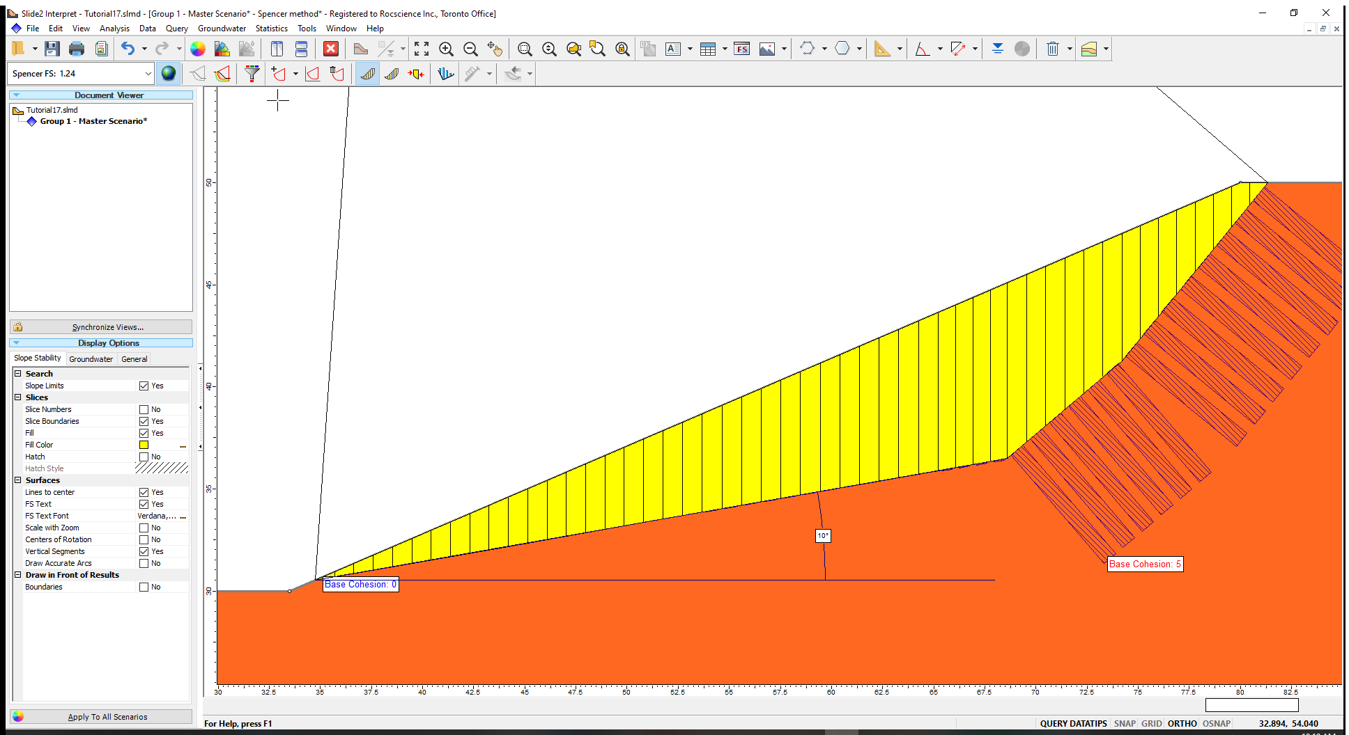
This shows the importance of using a non-circular failure surface in anisotropic models since the failure surface ‘seeks out’ the weak bedding orientation to yield a lower factor of safety.

5.0 Anisotropic Surfaces

Now we will try to define an anisotropic surface to define the anisotropy instead. This can be useful when modeling bedded materials.

Return to the Modeler and duplicate the group we have defined:

1. Right-click on Group 1 in the Document Viewer.
2. Select Duplicate Group.
3. Right-click on Group 2 and select Rename.
4. Name Group 1 “Angle” and Group 2 “Surface.”

We’re going to import a DXF file of a bedded material region:

5. Select File > Import > Import DXF . Select Tutorial 17 Bedding.dxf from the Tutorials folder.
   
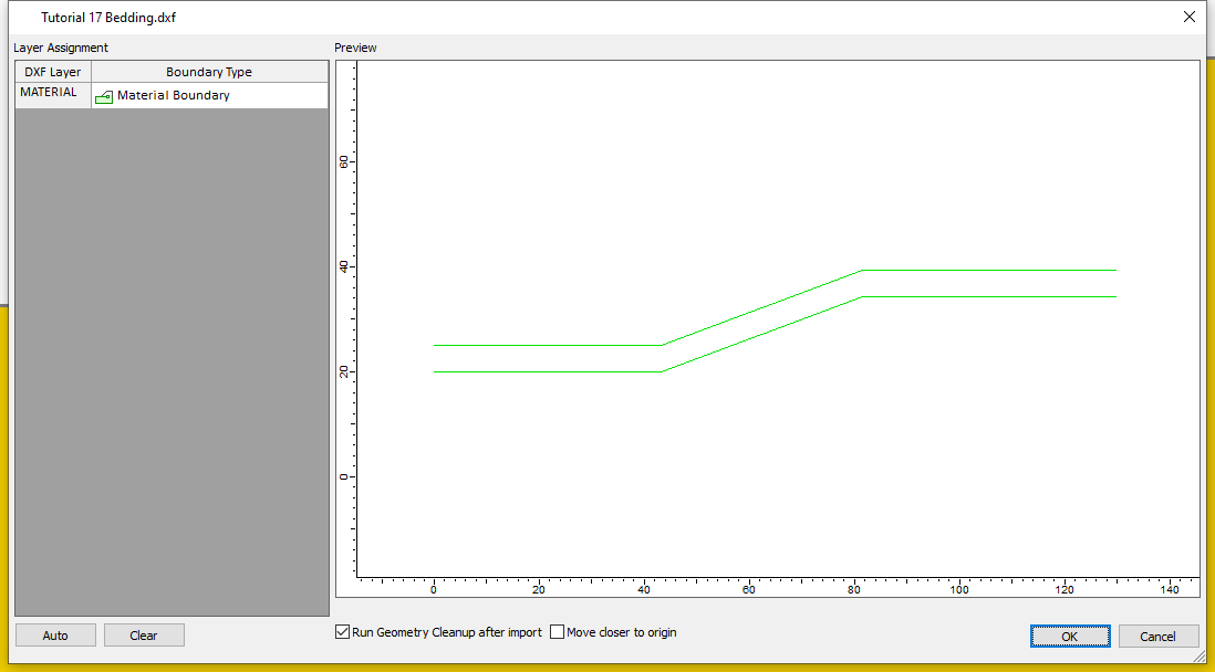
6. Click OK in the DXF Import dialog.

Now we’re going to define an anisotropic surface along this bedded region:

7. Right-click on the top material boundary and select Copy Boundary .
8. Click on the leftmost point (0, 25)
9. Input the new point in the command prompt: (0, 22.5).
10. Now right-click on the middle boundary (the one we just copied) and select Convert Boundary > Anisotropic Surface.
11. Now, assign the Soil Mass material around this boundary by right-clicking above it and selecting Assign Material > Soil Mass. Do the same below the boundary.
    

Your model should look as shown:

Let’s change the material properties for this region:

12. Select Properties > Define Materials
13. Click on Material 4 and name it Anisotropic Surface.
14. Set the Strength Type = Generalized Anisotropic and the Input Type = Angle or surface.
15. Click the pencil icon.
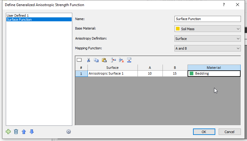
16. Add a new function by clicking on the green plus button on the bottom left. Input the following information:
• Name = Surface Function
• Base Material = Soil Mass
• Anisotropy Definition = Surface
• Joint Definition:
• Surface = Anisotropic Surface 1
• A = 10
• B = 15
• Material = Bedding



17. Click OK. The Generalized Function will now be the Surface function.
18. Click OK in the Material Properties dialog.
19. Right-click on the orange material and select Assign Material > Anisotropic Surface.

6.0 Compute & Interpret

1. Save the model by selecting File > Save As in the menu.
2. Select Analysis > Compute in the menu to perform the analysis.
3. Then select Analysis > Interpret to view the results.

As we can see in this case, the slip surface tries to follow the anisotropic boundary. Instead of comparing the base angle of the slice to the input angle as we did in the first group, it is now being compared to the angle of the segment of the anisotropic surface that is closest to the base of the slice.

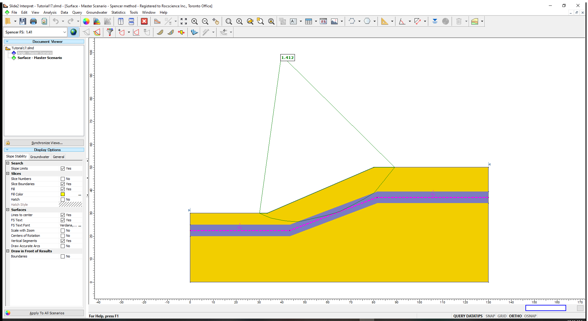
If we plot the Base Cohesion again (described in Section 4.0), we can see that the portion of the slip surface that is intersecting the purple region, and is aligned with the anisotropic surface, is taking the bedding cohesion of 0: