15 - Levee with Toe Drain

1.0 Introduction

In this tutorial, we will use Finite Element Groundwater Seepage analysis to evaluate the effectiveness of a horizontal toe drain constructed in a levee. Toe drains are used to prevent capillary rise on the downstream slope surfaces of embankments.

The finished product of this tutorial can be found in Tutorial 15 Levee with Toe Drain.slmd data file. All tutorial files installed with Slide2 can be accessed by selecting File > Recent Folders > Tutorials Folder from the Slide2 main menu.

2.0 Model Geometry

1. Select File > Recent Folders > Tutorials Folder in the Slide2 main menu.
2. Open Tutorial 15 Levee with Toe Drain - starting file.slmd.

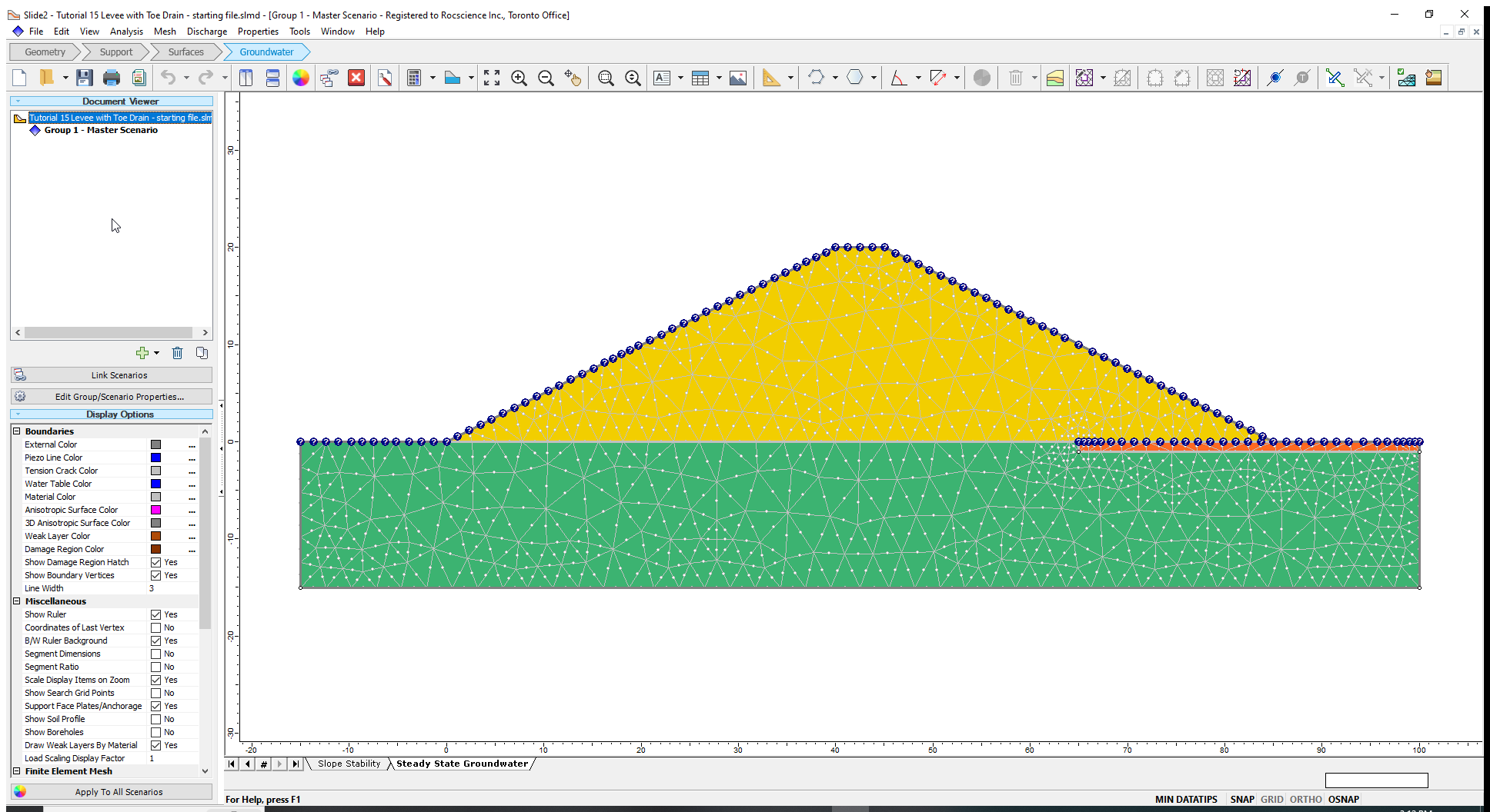
The following settings have already been defined for the model:

• The finite element analysis option is selected under the Groundwater tab of Project Settings. (See Analysis > Project Settings to view the option setting.)
• Materials have been named and assigned appropriately.
• Hydraulic properties of materials are defined. The underlying soil material is deemed to be impermeable. (View these parameters under Properties > Define Hydraulic Properties )
• The model is already meshed using 6-noded elements. (The settings can be reviewed under Mesh > Mesh Setup )

With these settings and parameters already specified, the next step is to set the groundwater boundary conditions.

2. Go to the Groundwater workflow tab

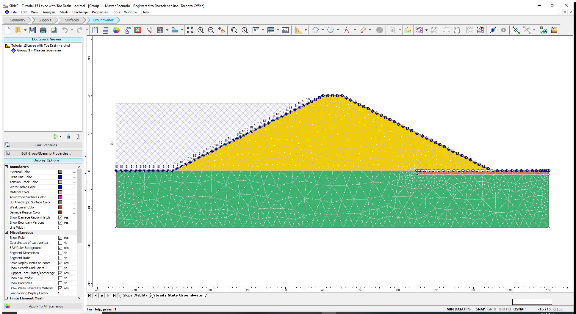
We will simulate ponded water at a depth of 18m to the left of the levee, i.e., set the total head to 18m.

3. Go to Mesh > Set Boundary Conditions to open the Set Boundary Conditions dialog shown below.
4. For BC Type, select Total Head (H) from the list.
5. Enter a Total Head Value of 18.
6. Ensure the Selection Mode is set to Boundary Segments
   
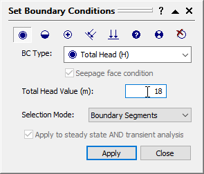
7. Select the two upstream boundary segments with the coordinates:
• Line 1: from (-15,0) to (0,0)
• Line 2: from (0,0) to (36,18)
8. Click Apply to attach this boundary condition to the selected line segments.

For the downstream side of the model, we will assume that the toe drain provides a drained boundary such that the groundwater pressure along the drain is 0.

We will apply Zero Pressure as the boundary condition for the top horizontal line segment of the toe drain.

9. Change the BC type to Zero Pressure and apply it to the boundary segment with coordinates (65,0) and (85,0).
   
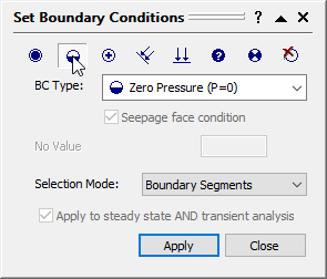
10. Click on the Apply button to assign the zero-pressure boundary condition.
11. Click Close to exit the dialog.

TIP: You can also right-click on a boundary to define its boundary conditions.

Now we are ready to compute the analysis. Since we are interested in only the groundwater results, we will run steady-state groundwater analysis only.

3.0 Computation and Interpretation of Results

1. Go to Analysis > Compute (groundwater) . This analysis will take a few seconds to run.
2. Select Analysis > Interpret (groundwater) to view the results.

The Pressure Head contours are displayed by default as shown in the image below.

For easy interpretation of results, let us turn on the material boundaries.

3. Go to View > Display Options to open the Display Options dialog.
4. Under the General tab, select the material boundaries checkbox.
5. Click Done to close the dialog.

The material boundaries will now be visible on the model as shown on the image below.

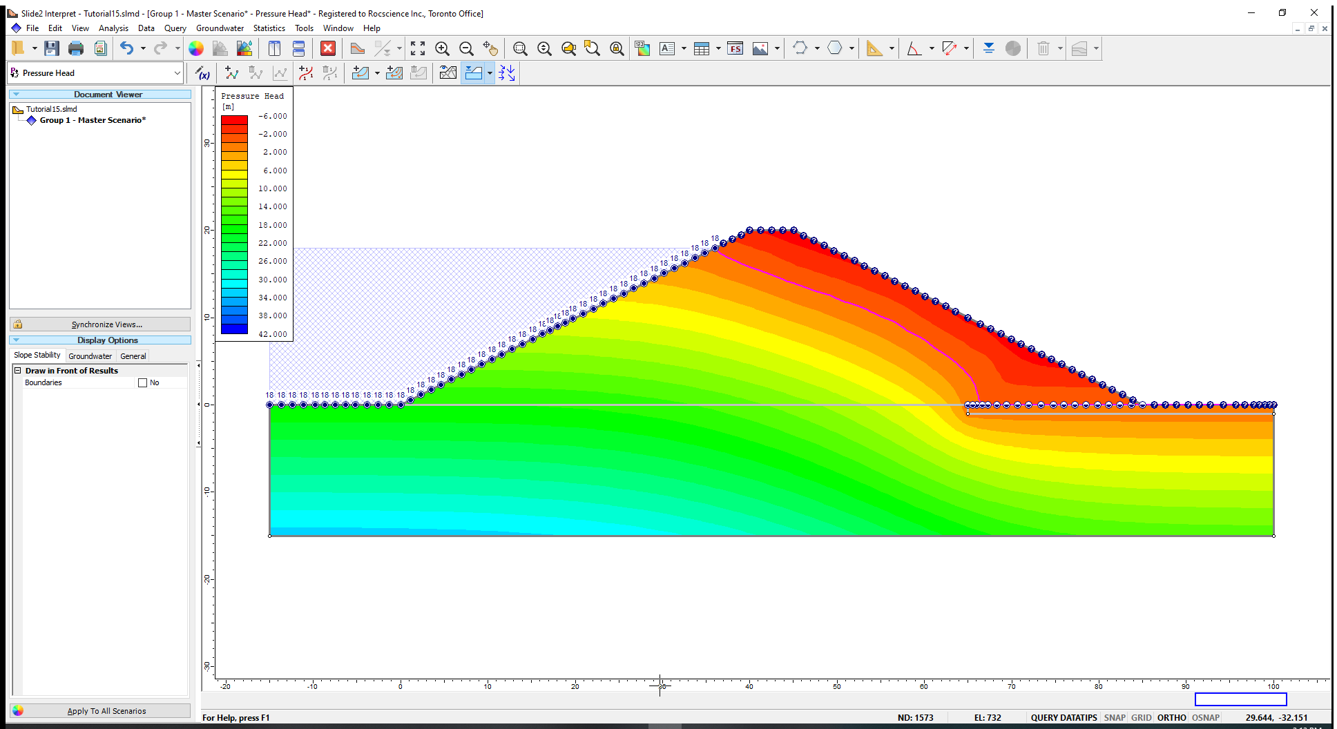
The purpose of the toe drain is to prevent the phreatic surface from intersecting with the downstream (right) face of the embankment. The phreatic surface (which is the pink line on the plot) resulting from the analysis does not touch the downstream face. This phreatic surface location indicates that the drain is performing as desired.

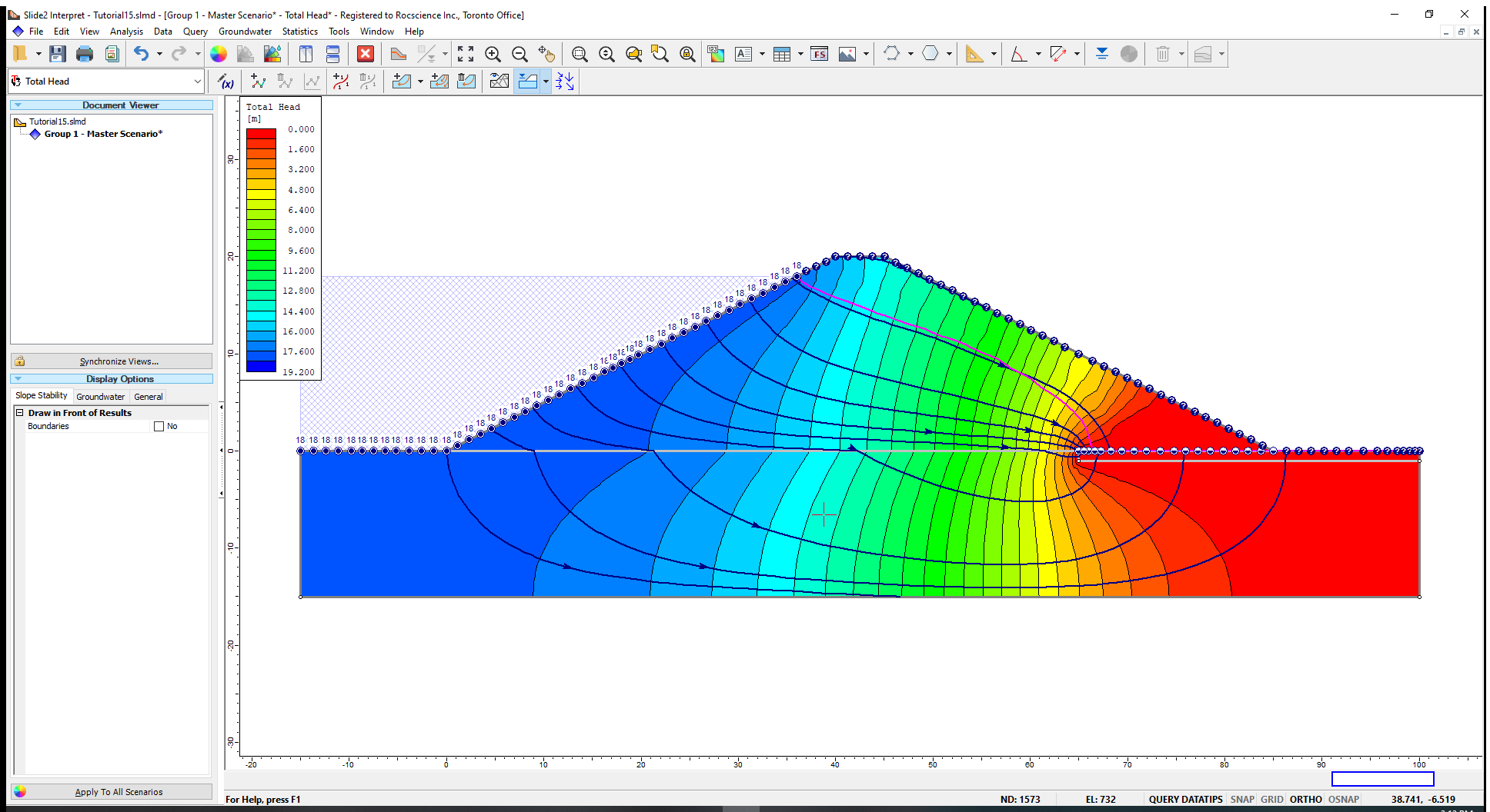
To examine the results in further detail, we will construct a flow net, which comprises equipotential and flow lines. Flow nets are an important tool often used in seepage analysis to solve problems of flow in structures like dams or evaluate the validity of solutions obtained.

We will achieve our goal by first drawing equipotential lines followed by flow lines.

6. Click on the drop-down arrow in the contour box and change from Pressure Head to Total Head. (Total Head contours represent equipotential lines.)
7. Right-click on the model and select Contour Options to open the dialog.
8. In the Contour Options dialog, select Filled (with lines) under Mode.
9. Click Done to close the dialog and see the equipotential lines of the flownet shown below.

To construct the flow Lines:

10. Go to Groundwater > Lines > Add Multiple Flow-Lines
11. Select the top left corner of the levee (40,20) and the left corner of the levee (0,0).
12. Press the enter key to open the Flow-Line Start Location dialog shown below.
13. Under ‘Start Flow-Lines’ select the first option of ‘locations evenly spaced along the polyline’
14. Use the default value of 10.
    
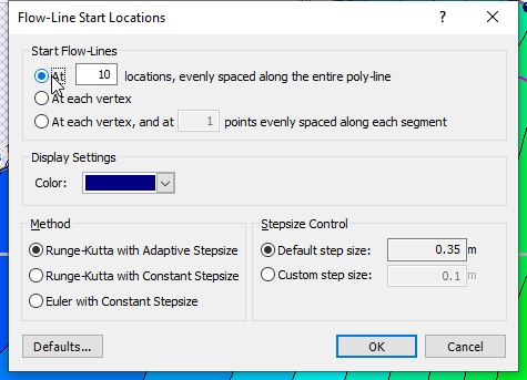
15. Click OK to close the dialog. Flow lines originating from the selected boundary are superimposed on the model results. The combination of the equipotential and flow lines creates the flow net shown below.

This concludes the Levee with Toe Drain tutorial.

4.0 Modelling Comments

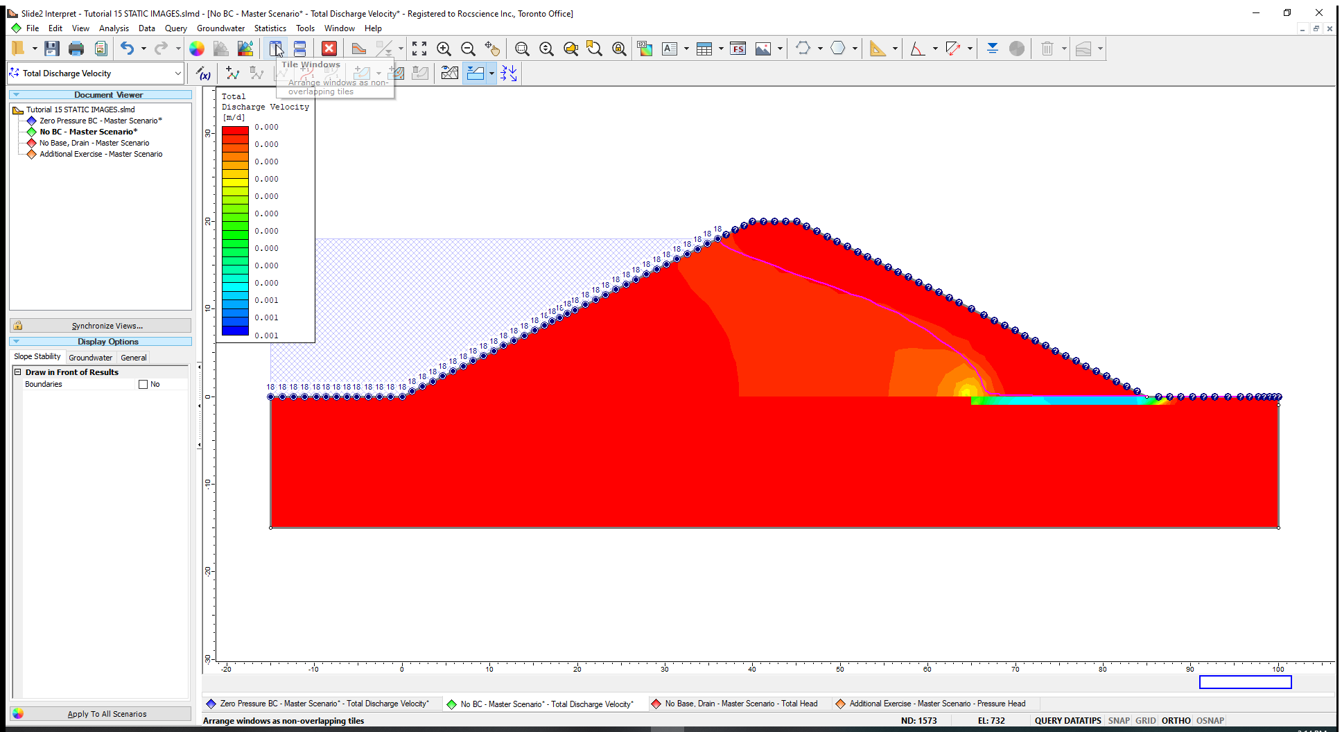
If you display the flow vectors for this model and view the discharge velocity contours (see figure below), you will observe that there is apparently no flow taking place within the drain material. This is because the zero pressure boundary condition along the top of the drain acts as a “sink” and is what stimulates the drainage condition.

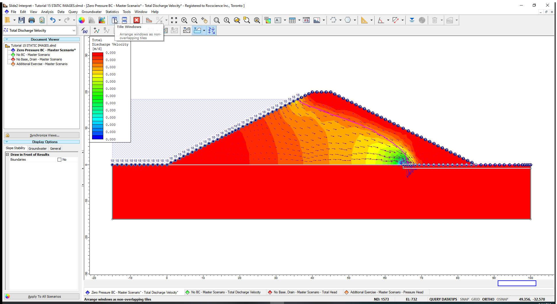
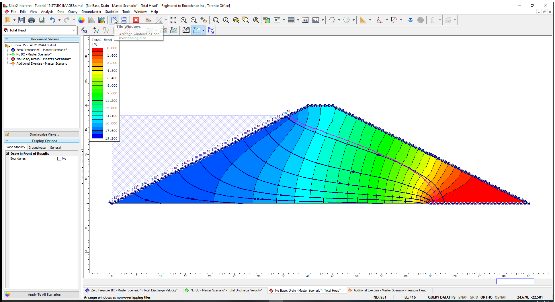
However, if you remove the zero pressure boundary condition at the top of the drain, and re-run the analysis, you will see actual flow through the drain material, as shown in the figure below. This behaviour, which is like that previously seen, is due to the high permeability of the drain, particularly when compared to that of the levee materials.

The similarity between the results of the different approaches will not always be the case, and in general, it is recommended that the zero pressure boundary condition be used to enforce the drainage condition at the desired location. However, the second approach can be used to determine the hydraulic conductivity that a drain needs to have to work as desired by the designers.

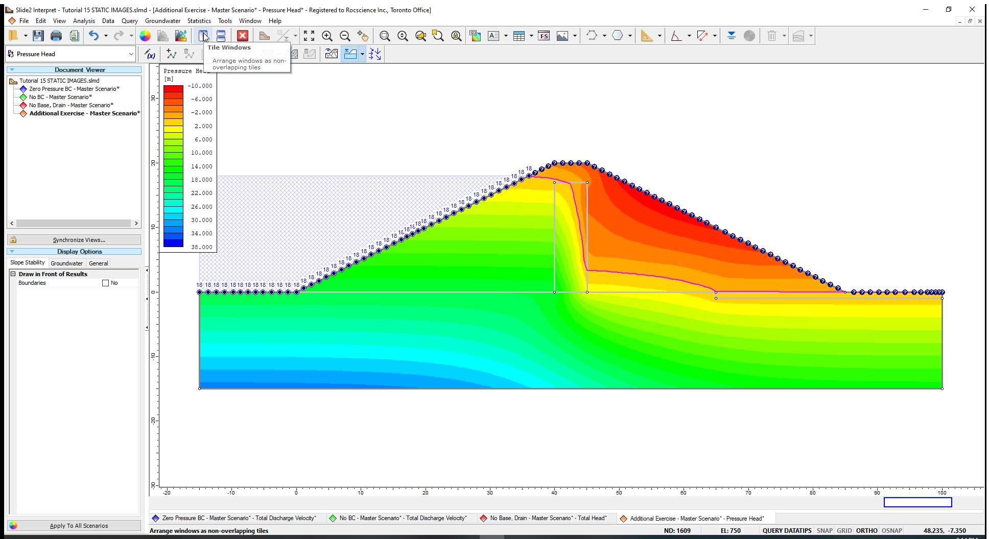
Another modelling alternative is to exclude the base and drain material altogether, and just model the levee material with boundary conditions, as shown in the next figure.

If you are only interested in groundwater results, and the base material is assumed to be impermeable, then it is sufficient to only model the levee as shown in the above figure.

However, if you are also carrying out a slope stability analysis, then you might require the base material to ensure a complete slope stability analysis of the entire model (i.e., to account for slip surfaces that pass through the base material).

5.0 Additional Exercises

We can simulate a levee with a low permeability core by specifying material boundaries to define the core and setting up new material with a lower permeability (say 1e-11 m/s). An example is shown below:

Another possibility is to construct a levee with a non-horizontal toe drain as shown below.

This type of model is described in Groundwater Verification Problem #4.