23 - Statistical Correlation

1.0 Introduction

This tutorial will demonstrate the statistical correlation options in Slide2, which allow you to equate or correlate material properties between different materials in a probabilistic analysis. At the end of the tutorial, we will know how to:

1. Statistically correlate material properties
2. Statistically equate materials

The finished product of this tutorial can be found in the Tutorial 23 Statistical Correlation.slmd data file. All tutorial files installed with Slide2 can be accessed by selecting File > Recent Folders > Tutorials Folder from the Slide2 main menu.

2.0 Model

For this tutorial, we will read in the starting file.

1. Select File > Recent Folders > Tutorials Folder from the Slide2 main menu.
2. Open Tutorial 23 Statistical Correlation – starting file.slmd.

This problem is modified from an analysis of the excavated slope for reactor 1 at Bradwell (Duncan and Wright, 2005 and Skempton and LaRochelle, 1965).

3.0 Material Properties

The slope is made up of three materials: Clay Fill, Marsh Clay, and London Clay (brown and blue). The undrained shear strength in the London Clay (brown and blue materials) increases non-linearly.

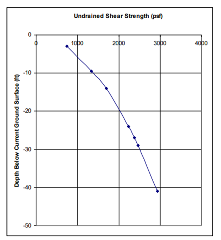
This has been estimated by dividing the brown and blue materials into several sub-materials which have linearly increasing cohesion. There is also a tension crack defined in the Clay Fill material.

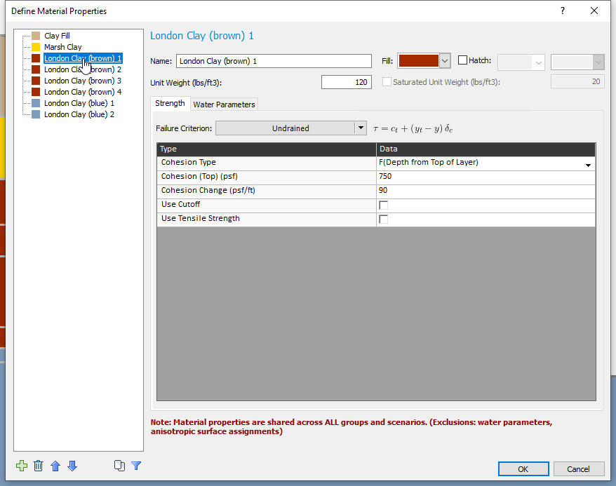
1. Select Properties > Define Materials
   
2. Click through the different materials to see the different properties. Notice that the London Clay materials are defined with linearly increasing cohesion via a Cohesion (Top) value and a Cohesion Change value.

We will turn on probabilistic analysis:

3. Close the Define Materials dialog and select Analysis > Project Settings Go to the Statistics tab.
4. Tick the checkbox to turn on Probabilistic Analysis.
5. Set the Number of samples to 100.
6. Change the Analysis Type to Overall Slope. This means that an independent search will be done in every simulation.
   
   
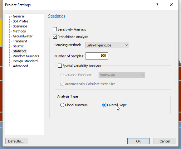
7. Click OK.

Now, we will define the statistical properties. We want to consider a range of Cohesion and Cohesion Change values in the brown London Clay material. That way we can see the impact on the factor of safety in case our measurements are not completely accurate.

8. Select Statistics > Materials
9. Select London Clay (brown) 1 on the left.
10. Click the Add button and select Cohesion and Cohesion Change.
    
    
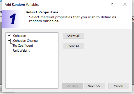
11. Click Next.
12. Keep Statistical Distribution as Normal.
13. Click Finish.

We want to consider a coefficient of variation (COV = Std.Dev/Mean) of 0.3 for Cohesion and 0.1 for Cohesion Change:

14. For Cohesion, input a standard deviation of 225.
15. For Cohesion Change, input a standard deviation of 9 .
16. Then click on each row and click the 3x standard deviation button on the right-hand side which will fill in the relative min and max with default values of 3.0*standard deviation.
    
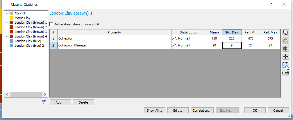
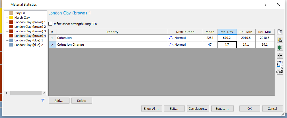
17. Repeat these steps for London Clay (brown) materials 2, 3, and 4, using the inputs in the table:

	London Clay (brown) 2	London Clay (brown) 3	London Clay (brown) 4
Cohesion Std. Dev.	400.5	511.2	670.2
Cohesion Change Std. Dev.	8.2	5.3	4.7

We don’t want the samples of Cohesion and Cohesion Change to be drastically different from each other, since what we really want to vary is the Depth vs. Undrained Shear Strength plot as a whole. Therefore, we will correlate Cohesion and Cohesion Change.

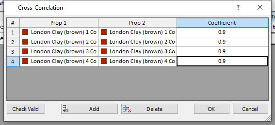
18. Select the Correlation button to view the Cross-Correlation dialog. In this dialog we can define correlation coefficients between any valid parameters of any strength type.
19. Click Add four times to create four rows.
20. Now adjust the properties such that each row contains Cohesion and Cohesion change for each material.
21. Enter a correlation coefficient of 0.9 for each row. The dialog should look as shown:
    
    
22. Click OK on the subsequent three dialogs. We are now ready to compute.

4.0 Compute

1. Save the model by selecting File > Save As in the menu.
2. Select Analysis > Compute in the menu to perform the analysis. Since we are performing an Overall Slope analysis, 100 separate limit equilibrium analyses are being computed. This may take a couple of minutes.
3. Then select Analysis > Interpret to view the results.

5.0 Interpret

The Interpret program shows the results of the Bishop analysis.

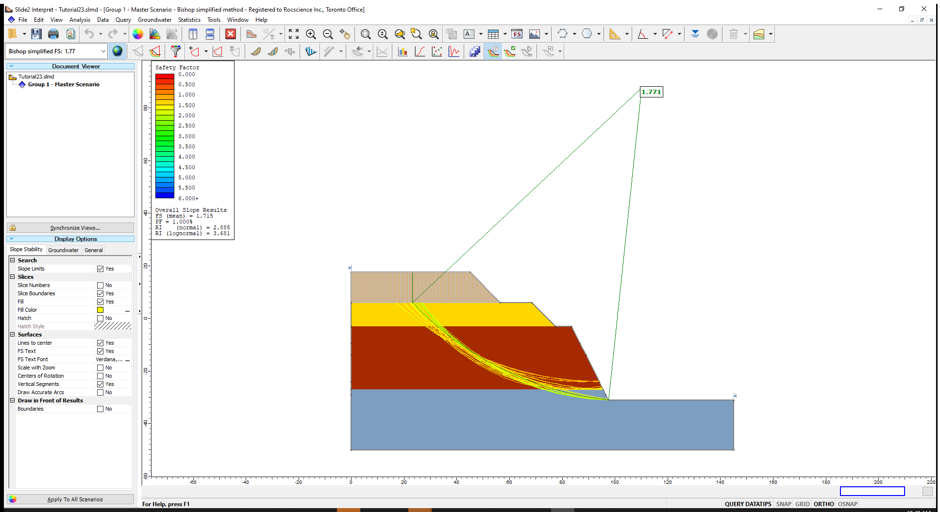
We can see all the critical global minima found in the 1000 analyses plotted on the slope. The probability of failure (PF) is found under the legend. The factor of safety shown is the one for the deterministic analysis.

Now let’s look at some scatter plots:

1. Select Statistics > Scatter Plot
2. Set the Horizontal Axis to London Clay (brown) 1: Cohesion.
3. Set the Vertical Axis to London Clay (brown) 1: Cohesion Change.
4. Click Plot.

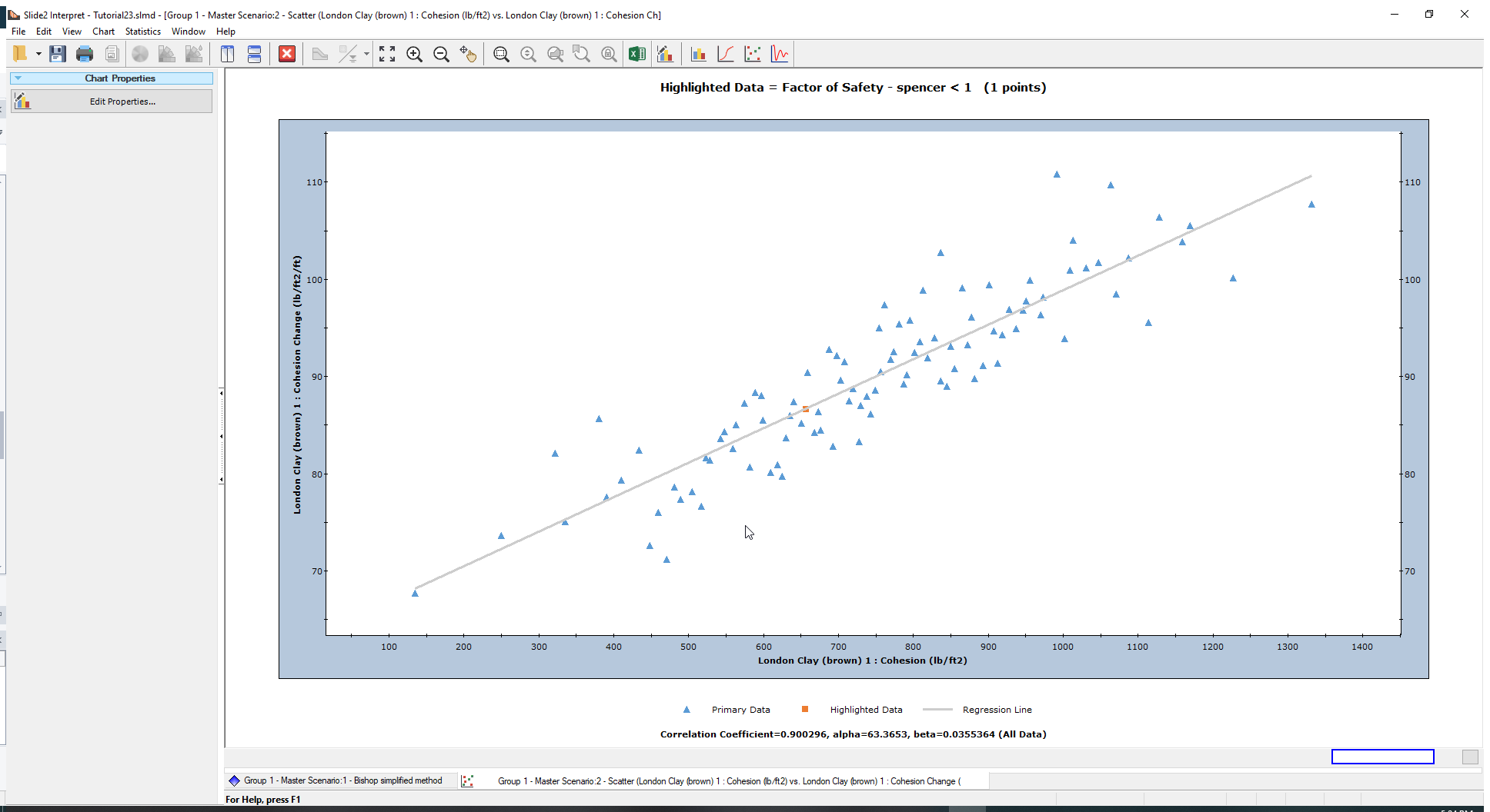
As expected, the Cohesion and Cohesion Change are closely correlated. For example, for a top Cohesion of approximately 1200 lb/ft2, the corresponding Cohesion Change in that simulation might be roughly 100 lb/ft2/ft, rather than something on the very low end such as 70 lb/ft2/ft.

Now let’s look at other data:

5. Right-click on the plot and select Change Plot Data
6. Change the Vertical Axis to London Clay (brown) 2: Cohesion.
7. Click Done.

We are now looking at the top cohesion of the first layer and second layer. Because these are sample randomly, we can see that there are some very odd simulations generated. For example, we can have a top cohesion in layer 1 of 900 lb/ft2, paired up with top cohesion in layer 2 of 600 lb/ft2. Hover over the points to see the coordinates and hence examples of such simulations.

This doesn’t make sense because the cohesion should be increasing with depth. Therefore, the analysis we have created is nonsensical. We need the second layer to have samples of Cohesion and Cohesion Change that change proportionally to the first layer in order to get a realistic Depth vs Undrained Shear Strength plot.

8. Go back to the Modeler.

6.0 Equating Materials

In the Modeler, let’s return to the Material Statistics dialog:

1. Select Statistics > Materials
2. Now click the Equate button to open the Equate Materials dialog.
3. Click Add Group.
4. In the wizard, click Select All to equate all four layers of the brown London Clay.
5. Click Next.
6. In the second step, click Select All to equate all probabilistic parameters in each material.
7. Click Finish.
   
   
8. The dialog will look as shown above. Click OK in the two subsequent dialogs.

What we have done, is that we have synced the London Clay (brown) materials completely. That means for example that if the cohesion of layer 1, sampled in simulation 1, is in the bottom left corner of the normal distribution, layers 2, 3, 4 will have a sample of cohesion in the exact same bottom left corner of their respective normal distributions. The same applies for cohesion change.

Let’s see the results.

9. Select Analysis > Compute
10. Then select Analysis > Interpret to view the results.

7.0 Interpret of Equated Materials

Now let’s look at the scatter plot again:

1. Select Statistics > Scatter Plot
2. Set the Horizontal Axis to London Clay (brown) 1: Cohesion.
3. Set the Vertical Axis to London Clay (brown) 2: Cohesion.
4. Click Plot.

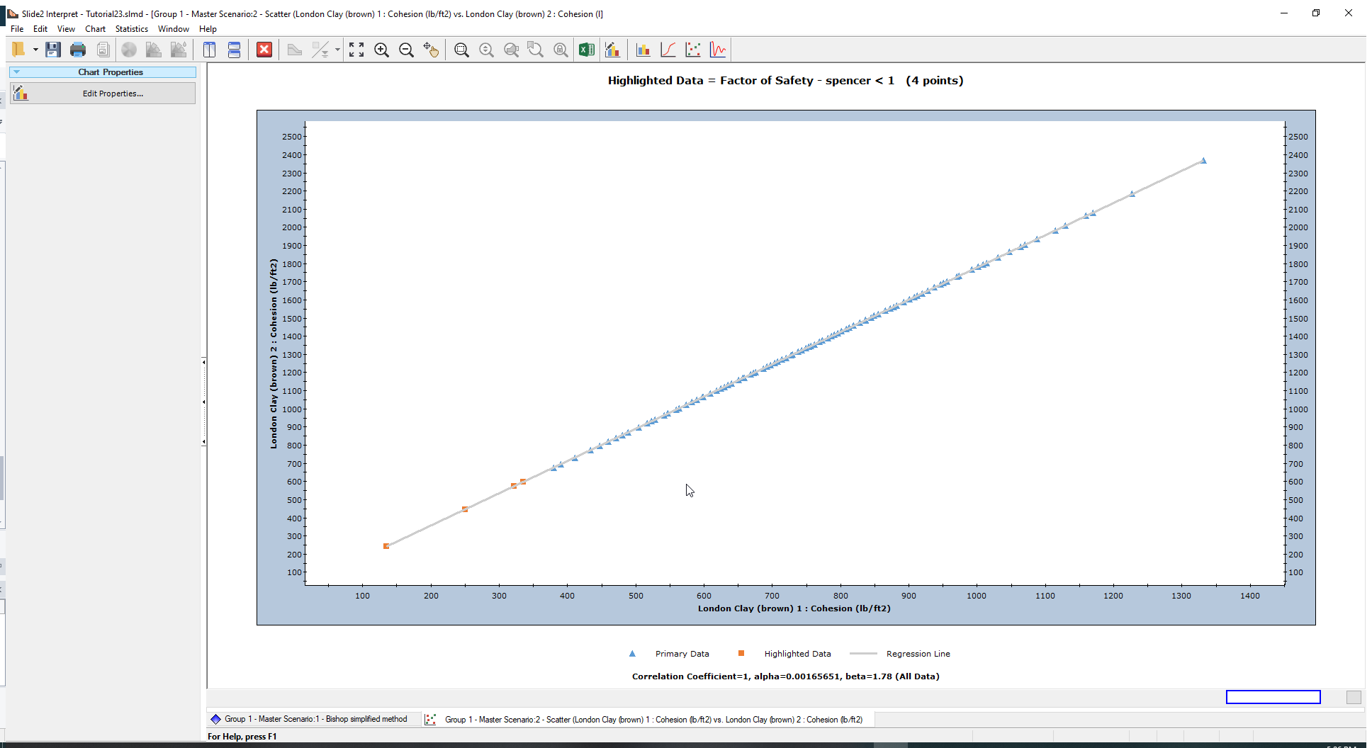
The values are now perfectly correlated. That means that if the cohesion of layer 1 is 900 lb/ft2 in a given simulation, the corresponding cohesion of layer 2 will be around 1600 lb/ft2. That way the top cohesion and the cohesion change are always increasing proportionally to the layers around them.

As an additional exercise, you can do the same for the blue London Clay material layers.

This concludes the tutorial.