RSPile Integration

1.0 Introduction

This tutorial is an extension of Slide2's RSPile tutorial. This tutorial will demonstrate how to determine pile forces on Slide3 and verify the pile resistance in RSPile.

The finished product of the Slide3 model can be found in Slide3 with RSPile (Final).slide3m2

2.0 3D Pile Analysis

The Slide3 integration of RSPile is similar to the integration in Slide2, except that there are several additional assumptions required to facilitate the additional dimension in space. For prerequisite information on pile resistance for slope stability analysis and RSPile, please visit Slide2-RSPile Tutorial as well as the RSPile Theory Manual.

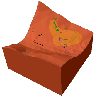
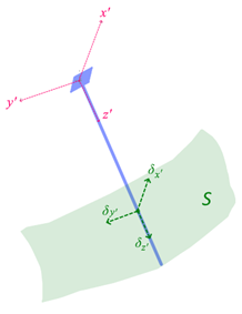
Like the 2D analysis, the soil displacement is split into axial and lateral components. However, in 3D the lateral soil displacement has components in both orthogonal local lateral axes in RSPile, X’ and Y’. As shown in the below figure, δ is the soil displacement caused by the slipping surface S at its intersection with the pile, which is resolved into components along the local axes of the pile, δ_x’ δ_y’ and δ_z’. As with the 2D analysis, the soil displacement is assumed to occur uniformly from the top of the pile down to the slip surface.

In RSPile, the analysis of soil displacement is conducted independently along each of the local axes. As such, some parameters originally used for 2D pile analysis such as the ground slope and batter angle are determined in each of the local axis directions separately. By default, this is done automatically between Slide3 and RSPile. For more information on how this is accomplished, refer to the last section of this tutorial. Like the 2D analysis, computations for the pile reactions are completed prior to the searching of slip surfaces in Slide3. Varying displacements in all three local directions are assumed at certain points along the pile, and the resulting reactions from the pile are pre-calculated for each case. Then during searching of the critical factor of safety in Slide3, the components of the pile reaction in each of the three local directions is interpolated from these results based on the sliding direction and intersection of the slip surfaces with the pile. There will be a verification exercise at the end of this tutorial which will be used to demonstrate this process in more detail.

3.0 Model

3.1 Import Model

To import the Slide2 Tutorial 30 model:

1. Select File > Import > Import Slide Project and navigate to the Slide3 Tutorial folders.
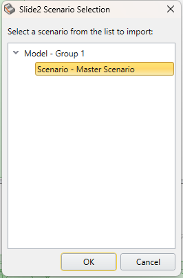
2. Open Slide file for importing.slmd file from RSPile- starting file folder. You will be prompted to select a scenario from the list to import.
3. Select Scenario – Master Scenario and click OK.
   
   
   
   
   
4. After selecting ‘OK’, the Import Slide2 Project prompt will appear. Change the extrusion depth to 260 m and click OK. A prompt may appear notifying you how the import/export process operates. Click OK.
   
   
   
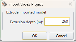
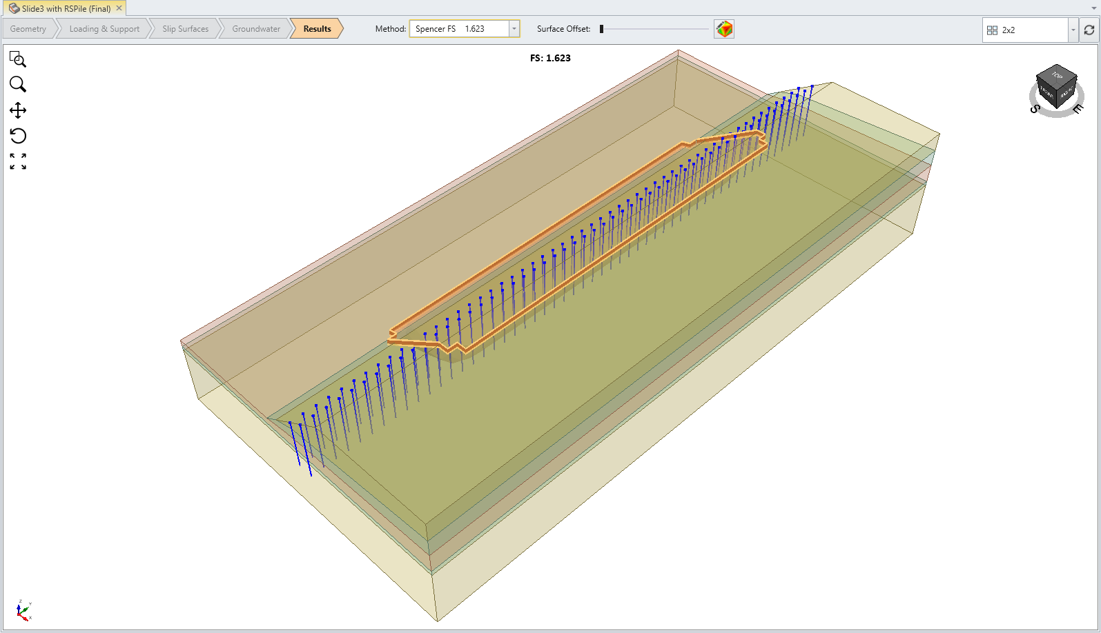
   You should see the following 3D model. This is identical to Slide2 tutorial 30’s model but extruded 260 m in the Y-direction.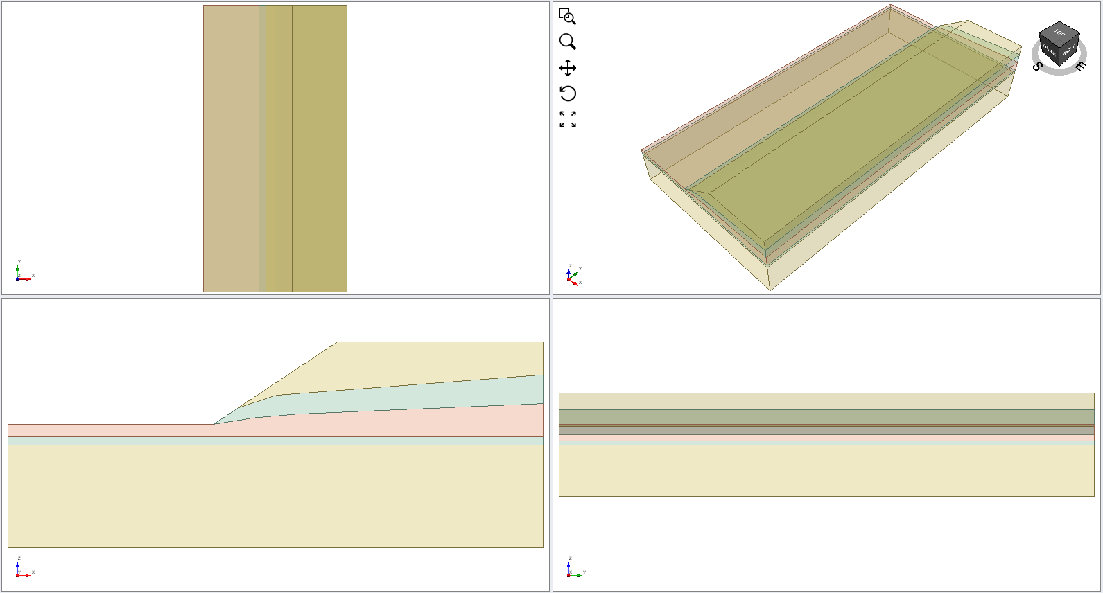
   
   

Note that the piles are also imported from the Slide2 file. To make the piles visible go under the Loading & Support tab.

3.2 Surfaces

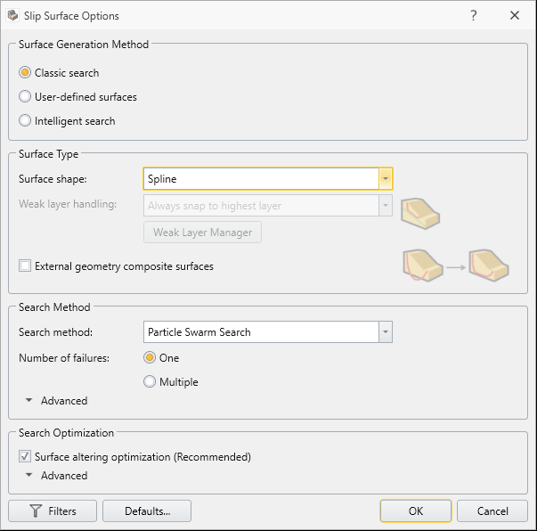
1. Select Surfaces > Slip Surface Options.
2. We will use Spline surface search with Surface Altering Optimization.
   
   
   
   

3.3 Support Properties

To define the pile properties, we must import the RSPile file.

1. Select Support > Define Support
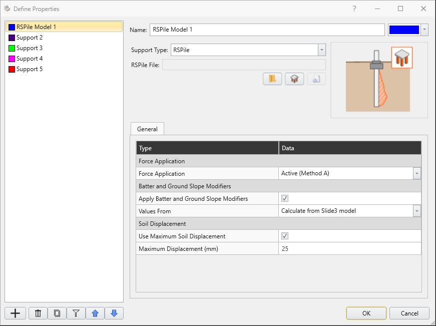
2. The Define Support properties dialog should appear. Verify that the properties are defined as:

• Name = RSPile Model 1
• Support Type = RSPile
• Force Application = Active (Method A)
• Apply Batter and Ground Slope Modifiers = Yes
• Ground Slope and Batter Values = Calculate from Slide3 model
• Soil Displacement Type = Maximum (Method A)
• Soil Displacement = 25 mm
  
  
  
  
  

3.4 Importing RSPile Model into Slide3

1. When RSPile is selected as the Support Type, the RSPile File section becomes visible. Select Choose File and import Analyzing Pile Resistance using RSPile (Starting File).
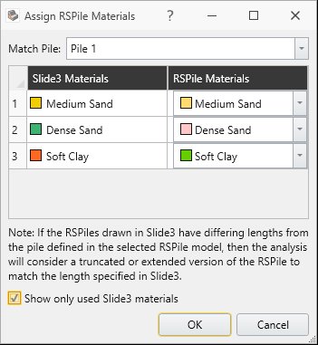
2. The following dialog should appear. Check 'Show only used Slide materials' at the bottom and ensure that each material in Slide3 is matched with the same material in RSPile. Click OK.
   
   
   
   
3. Click OK in the Support Properties dialog.
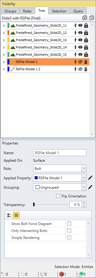
4. Verify that two created rows of supports have the applied property of “RSPile Model 1”.
   
   
   
   

4.0 Interpret

1. Save the file and Compute
   The search for slip surfaces may take several minutes. Alternatively, you can open the final file to review the results: Slide3 with RSPile (Final).slide3m2
2. When the computed results are available, click on the Results workflow tab.
3. In the tool bar, ensure that ‘Show Intersecting Bolts’ is selected. This option only shows piles that intersect the critical slip surface.
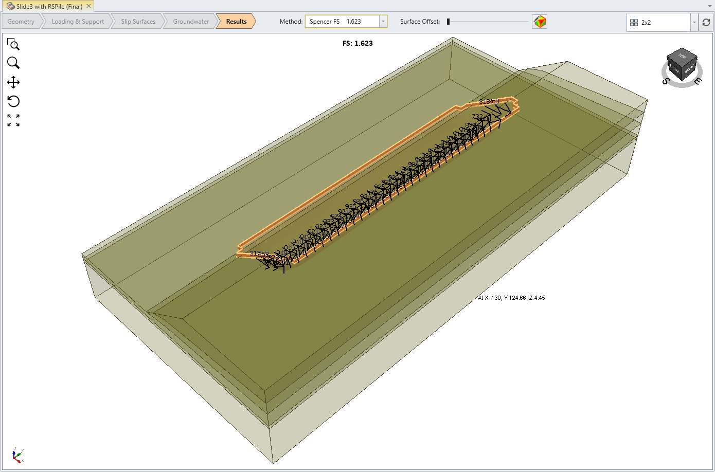
4. Switch to the Spencer FS results. You should see the following model under the Spencer FS analysis.
   

4.1 Pile Resistance

There are two ways to view the pile resistance forces:

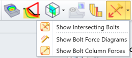
1. Click on the dropdown for bolts in the top menu as shown below and select Show Bolt Column Forces
   
   
   
   
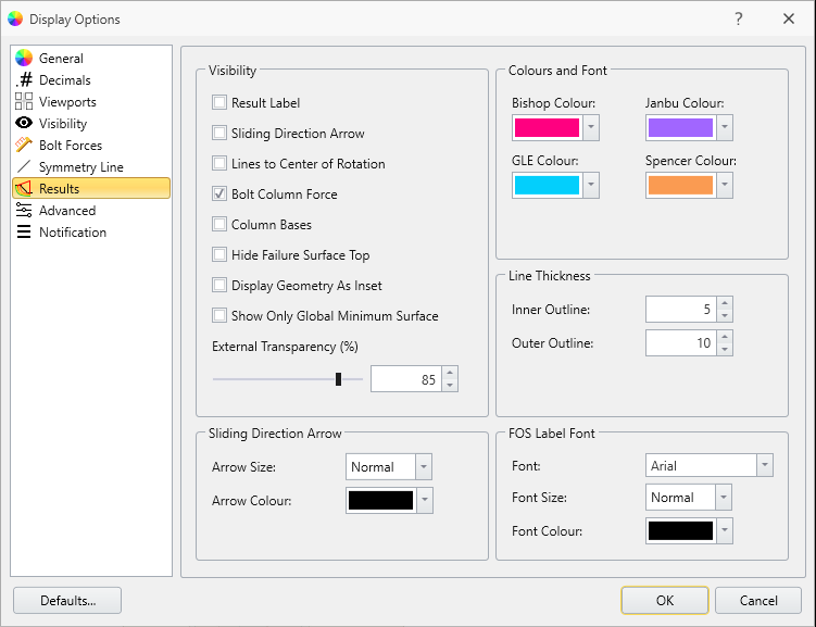
2. Alternatively, select: Interpret > Results Display Option. Under the Results tab, select Bolt Column Force.
   
   
   

All the pile resistance forces will now be displayed. Notice how the direction of each pile opposes the slip direction.

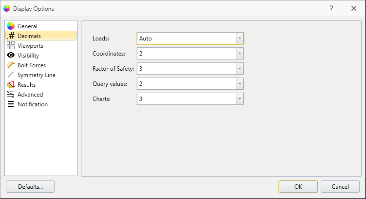
4.1.1 Change Decimals

1. In the Display Options dialog, select the Decimals tab and change the number of decimals for Loads to Auto.
2. Click OK.
   
   
   
   
3. Ensure that the visibility of the piles is turned on in the Visibility Tree (the icon should be displayed next to the bolt elements).
   
   
   
   

5.0 Additional Exercise: Verifying Pile Resistance against RSPile

You can verify the pile resistance results from Slide3 by using the same pile length and configuration from the RSPile model. As an additional exercise, you can verify the pile resistance for the downslope middle pile.

1. Start the RSPile program and open the RSPile File: Analyzing Pile Resistance using RSPile (Starting File)
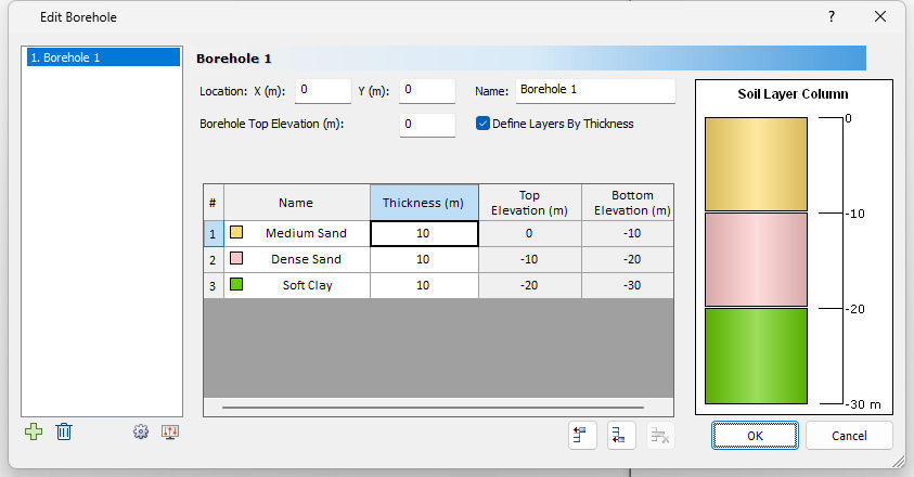
2. Go to Soils > Edit All Boreholes and ensure the soil layer thickness is the following:

Name	Thickness
Medium Sand	3
Dense Sand	5
Soft Clay	5
Dense Sand	2
Medium Sand	6

You can then follow the process for comparing the pile resistance is explained at the end of the Slide2-RSPile tutorial to see if the forces match between Slide3 and RSPile.

6.0 Further Discussion

Some additional technical details about the Slide3 integration of RSPile are addressed below.

6.1 Effective Ground Slope

The effective ground slope relates to the slope of the ground and angle of the pile in the lateral analysis, and is an optional parameter used to adjust the p-y curve during the pile analysis.

As the concept of an effective ground slope was originally intended for 2D pile analyses, the apparent effective ground slopes in x’ and y’ are determined separately using the following methodology.

The ground slope and batter angle for the piles can be calculated automatically based on the Slide3 model or specified manually in the RSPile file.

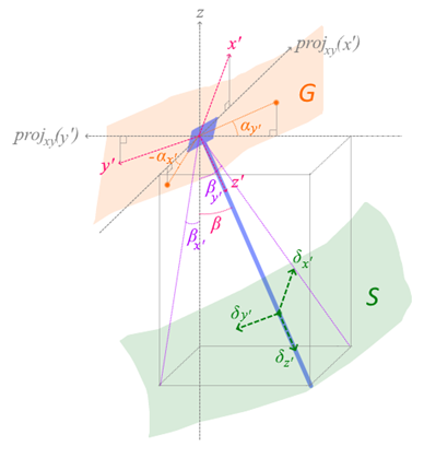
• α_x’ and α_y’ are the ground slope angles in each of the lateral (x’ and y’) directions, determined by the orientation of the ground topography G at the head of the pile. Note that for the purpose of illustration, proj_xy(x’) and proj_xy(y’) are directional vectors obtained by projecting x’ and y’ onto the horizontal (xy) plane, respectively. Ground slope is positive slanting downwards.
• β_x’ and β_y’ are the apparent batter angles in each of the lateral directions, and β is the true batter angle of the pile with respect to the vertical axis. The apparent batter angles are determined by projecting the pile onto the vertical planes containing x’ and y’, respectively, and then taking the angle of the resulting projection from the vertical. Batter angle is positive if the pile tilts always from the local axis.
• The effective ground slope angle in either x’ or y’ is taken as the ground slope minus the batter angle.