Probabilistic analysis - COV

1.0 Introduction

Probabilistic Analysis can be performed using Slide3 for various applications of slope stability. This tutorial covers a slope geometry with different complex material types including varying anisotropic materials assigned to the slope stability analysis. The objective of this tutorial is to introduce the use of Coefficient of Variation (COV) in Slide3 and the associated interpretation of the results.

The finished product of this tutorial can be found in the Tutorial 39 COV - Final file.Slide3m2 data file. All tutorial files installed with Slide 3 can be accessed by selecting File > Recent Folders > Tutorials Folder from the Slide 3 main menu.

2.0 Project Settings

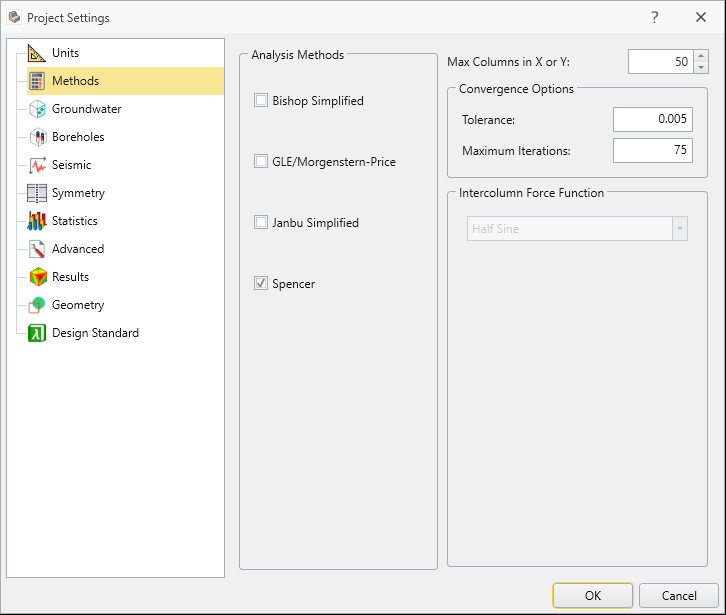
We will first check for methods.

• Open the Project Settings dialog from the toolbar or the Analysis menu
• Click on Methods to see that the Spencer method is selected
  
  

3.0 Model

1. Select Materials > Define Materials

You will notice that the yellow material is a Shale with a Shear/Normal Function strength type.

2. You can click the Pencil icon to see the Shear/Normal function.
   

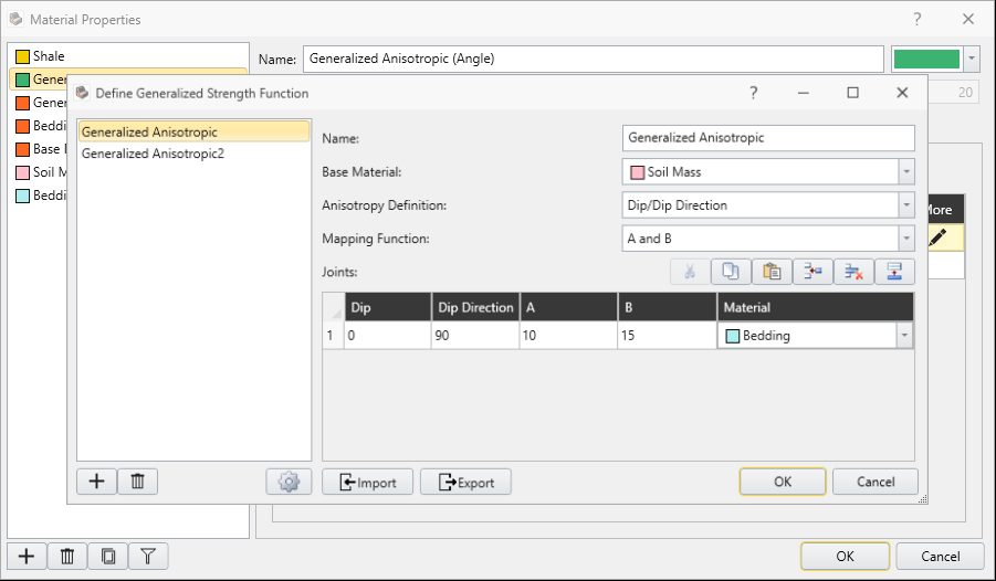
There is also the green material, Generalized Anisotropic (Angle), and red material, Generalized Anisotropic (Surface) using the Generalized Anisotropic as the Failure Criterion. If you click the Pencil icon, you will see that their strength function is defined by two other materials as shown below:

4.0 Compute

1. Save the file
2. Click Analysis > Compute to run the analysis
3. Select the Results workflow tab to view the results.

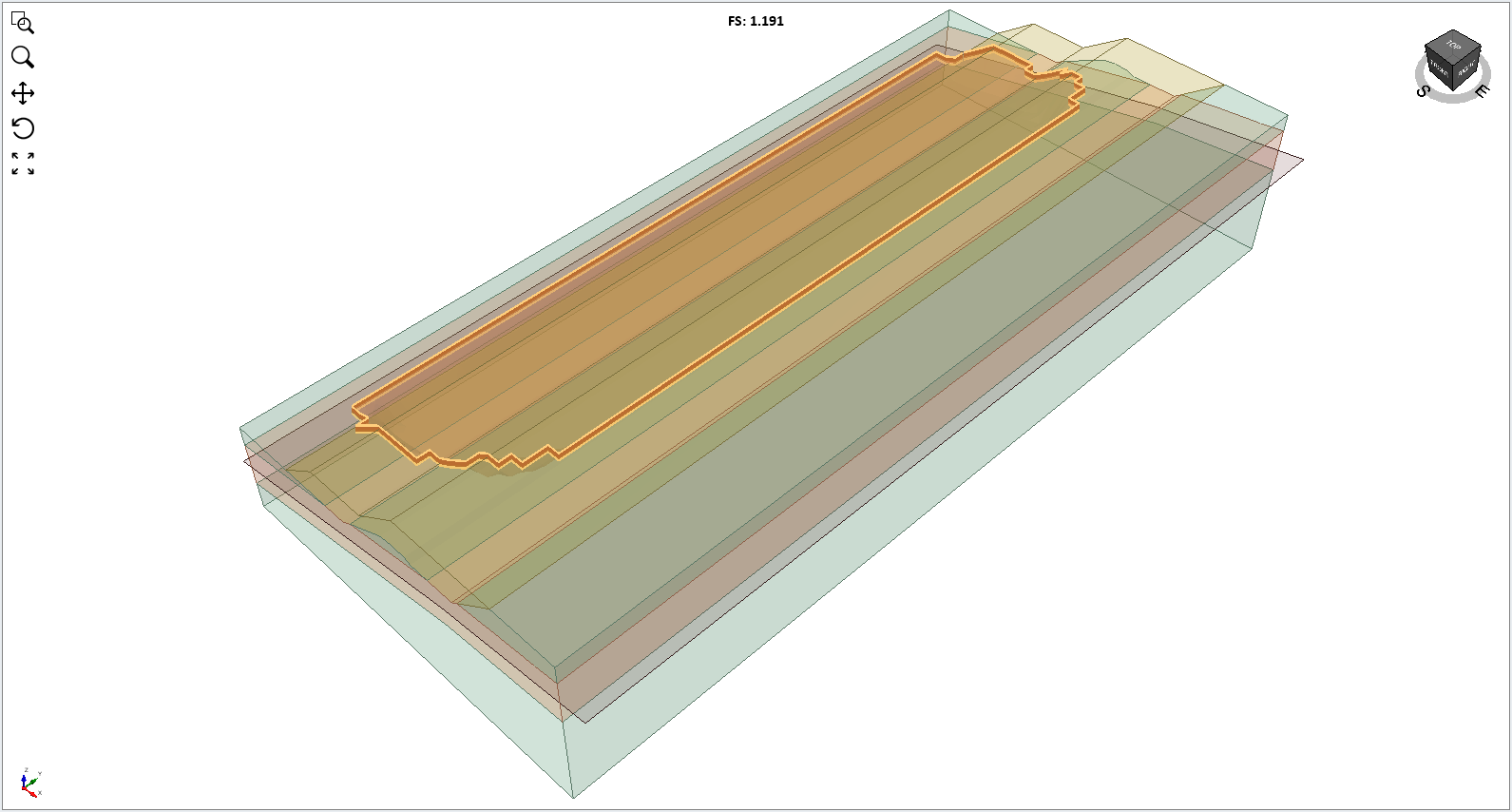
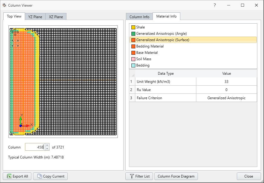
You will notice a minimum surface that intersects all three materials, with a Factor of Safety of about 1.2 as it can be seen in the column viewer option below:

5.0 COV OPTION

To use the COV option, we first must enable Probabilistic Analysis. To do this:

1. Select Analysis > Project Settings in the menu
2. Click on the Statistics tab
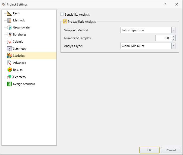
3. Check the Probabilistic Analysis box
4. Then set the Sampling Method to Latin-Hypercube, the Number of Samples to 1000 and the Analysis Type to Global Minimum as shown
5. Click OK
   
   



Now the Statistics menu will appear in the menu bar,

6. Select Statistics > Material statistics.
7. You will notice the Define shear strength using COV box. Check this to enable the option for the Shale material. You will see input fields appeared as shown:
   
   



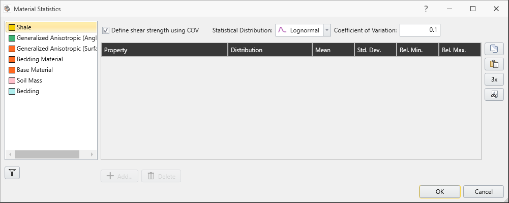
This means that the shear strength of the Shale will vary according to a Lognormal Distribution, with a coefficient of variation of 0.1. The coefficient of variation is defined as the standard deviation divided by the mean. Because the shear strength value changes according to location, the user only needs to define the standard deviation as a fraction of the mean.

8. Now select Generalized Anisotropic (Angle) material and check the COV box
9. Select a Uniform Distribution and change the range to 0.75 and 1.25:
   
   



The meaning of this is that in each simulation the shear strength value calculated at a given location will be multiplied by a value between 0.75 and 1.25. Hence, we are saying that the shear value determined by the material input parameters may not be exactly that, and we want to consider some plus/minus variability in the shear strength.

10. Select the Generalized Anisotropic (Surface) material and define the shear strength of this material as a random variable with Lognormal Distribution and a COV of 0.2.

Notice that you can also define random shear for Soil Mass and Bedding materials, which make up the Generalized Anisotropic material. Keep in mind that if you do so, these random variables will be independent of the random shear in Generalized Anisotropic, meaning they will not be derived from the Generalized Anisotropic material’s random shear.

We will stick with these three random variables.

11. Click OK
12. Select Analysis > Compute and then OK in the dialog to proceed.

6.0 Results

If you look at the top toolbar in Slide3, you will see three result icons with statistics. Those can also be found by selecting:

Statistics > Histogram plot / Scatter plot / Cumulative plot.

We will first look at the histogram of this model.

1. Select Statistics > Histogram Plot
2. Select the Highlight Data and set the data to Factor of Safety - Spencer with comparison < 1
   
   
   
   
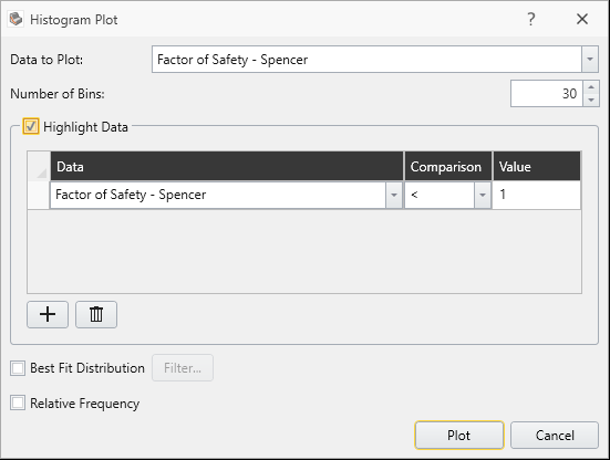
3. Click Plot, then you will see the following result with histogram shown below:
   

   
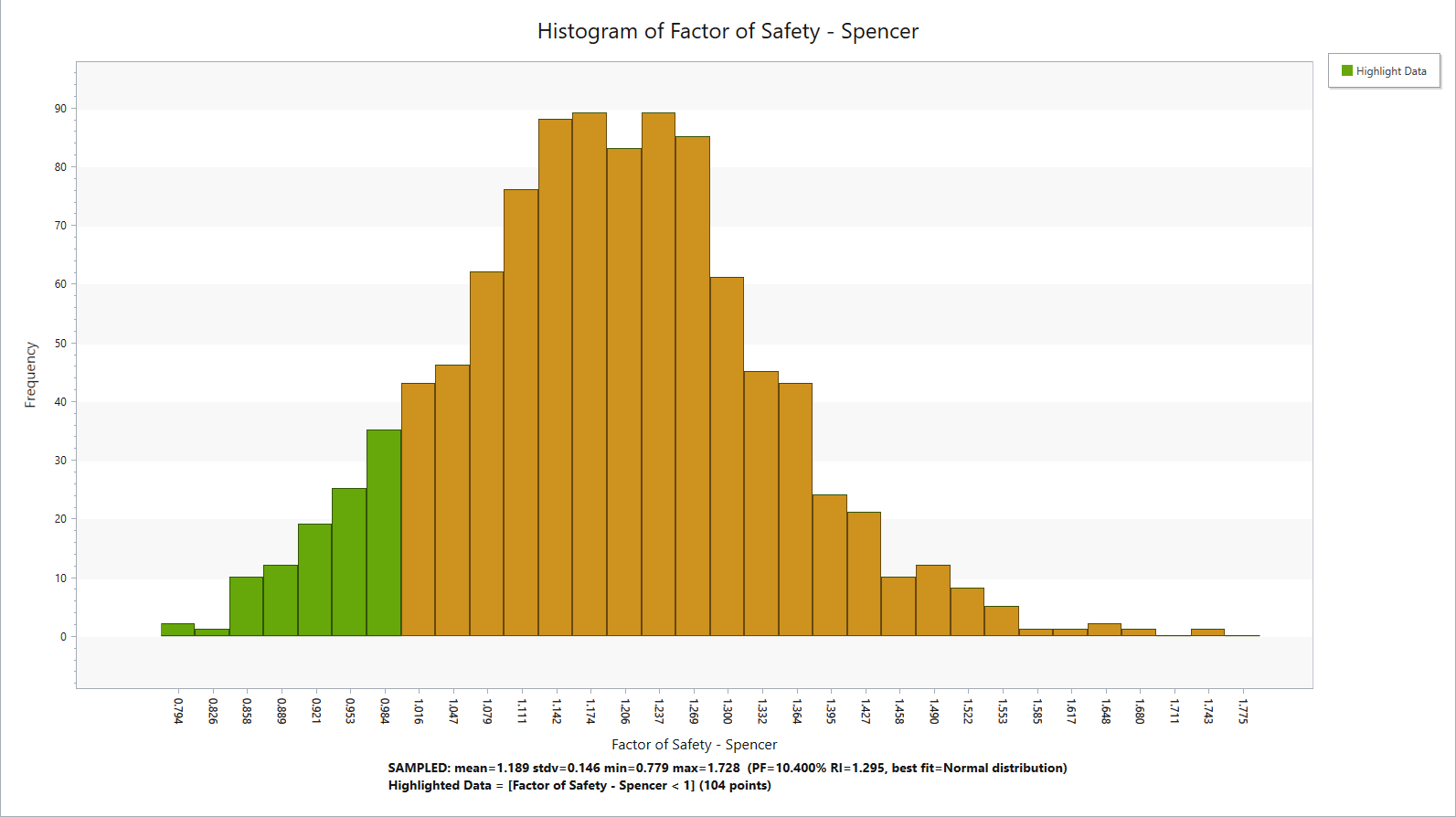
   As indicated in the graph, the highlighted sections are probability of failure where Factor of Safety was < 1 (with Probability of Failure = 0.5%).

   This can also be shown through scatter plot as well.
   
   

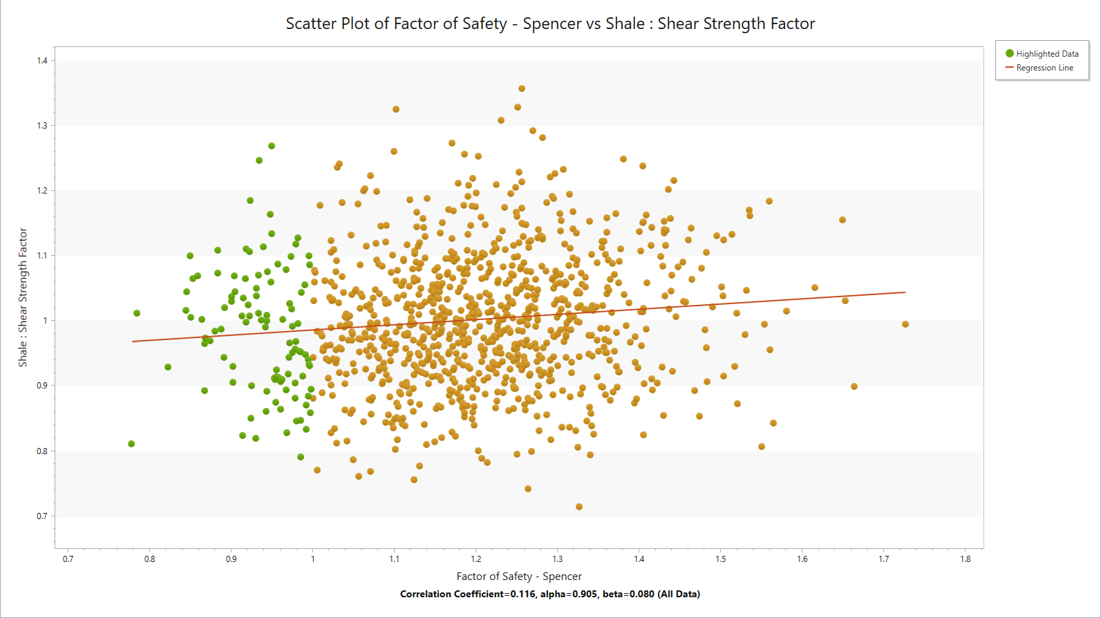
4. Select Statistics > Scatter Plot.
5. Select the Highlight Data and keep the values as default. (Factor of Safety - Spencer < 1)
   
   
   
   



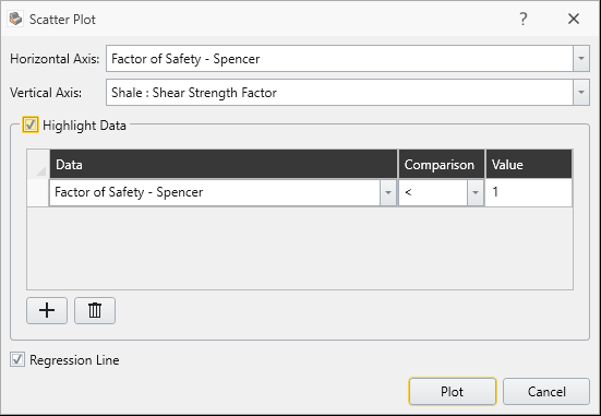
Here you see the scattered plot of Generalized Anisotropic (Surface).




Now we will look at the cumulative plot of the result.


6. Select Statistics > Cumulative Plot.
   
   



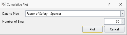
You will be prompted by this dialog.

7. Click Plot and you will see the cumulative Factor of safety for cumulative probability of failure as shown.
   
   

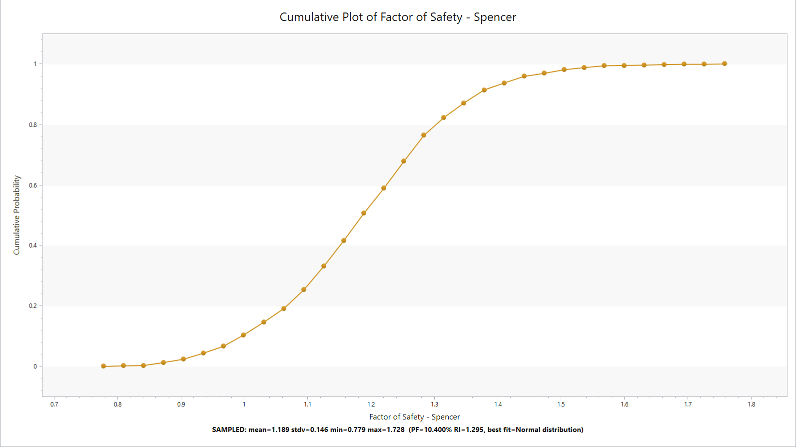
If you hover over to the Spencer FOS around 1, you can double check that probability of failure below FOS = 1 is around 0.5%.