Slope with Water Table

1.0 Introduction

The simplest 3D slope profile is one with a constant profile.

In this tutorial we will create a simple extruded slope, run the analysis, then add a water table and re-run the analysis.

2.0 Project Settings

Let’s first look at the Project Settings dialog. This allows you to configure the main settings for your analysis.

1. Select Analysis > Project Settings
   
2. Select the Units tab. Make sure the Units = Metric, stress as kPa.
3. Select the Methods tab. We will use the default selected methods (Bishop and Janbu)
   
   .
   
   
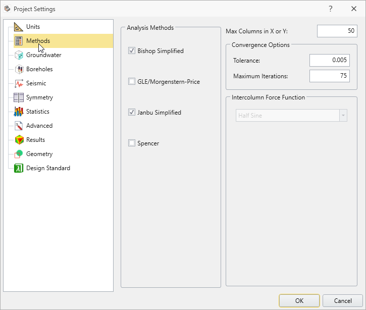
4. Select OK and close the Project Settings.
   

3.0 Geometry

1. Select the Geometry Workflow tab

For the purposes of this tutorial, we will create a 2D slope profile with the Draw Polyline tool using two different methods:

• Importing a .csv file, and
• Entering coordinates

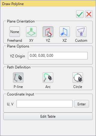
2. Select Geometry > Polyline Tools > Draw Polyline
   
3. We want to define the coordinates of the slope profile in the YZ vertical plane. Since the default setting is set to the XY plane, make sure to select the YZ Plane Orientation option in the sidebar on the left side of the screen.
   

3.1 Importing a .csv file

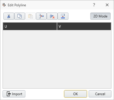
1. Select the Edit Table button in the Coordinate Input area of the sidebar.
2. The Edit Polyline dialog should open. You can import csv files by selecting Import
   
   
   
   
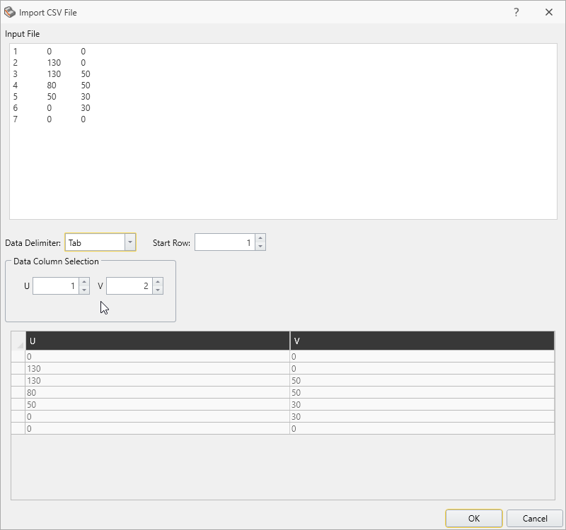
3. You should see the file 'polyline_coordinates.txt' in the tutorial folder. After you've opened the .txt file the Import CSV File dialog appears. Make sure to select Tab in the Data Delimiter dropdown.
4. You should now see a table of values. Click OK to go back to the Edit Polyline dialog.
   
   



Now we will delete the polyline coordinates and show how to enter the coordinates manually instead.

5. To delete the coordinates simply highlight the table and select the Delete Rows icon .

3.2 Entering Coordinates

1. In the Edit Polyline dialog, select the Append Rows button and add 7 rows, then click OK.
2. Enter the following coordinates in the dialog and select OK.
   
   

U	V
0	0
130	0
130	50
80	50
50	30
0	30
0	0

3. Click OK and close the Edit Polyline dialog, then select the green check mark at the top of the Draw Polyline dialog.
   
   
Alternatively, if you were working with the viewports you can right-click the mouse and select Done.
4. You have now added a 2-dimensional profile of a slope in the YZ plane. Press F2 to view the zoomed images of the polyline.
5. In the sidebar Visibility pane, select the Polyline entity you have just created.
   
   
   
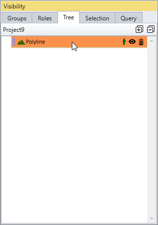
6. Below the Visibility pane (in the Properties pane) change the Name to Slope Profile.

3.3 Extrude

With the Slope Profile still selected we can extrude it to 3D.

1. Select Geometry > Extrude/Sweep/Loft Tools > Extrude
2. You will see the Extrude dialog. Select the Close Volume(s) checkbox at the top of the dialog. This ensures that the extruded volume will be closed (i.e. not open-ended).
   
   
The Direction is based on the plane of the slope profile. Since we defined the coordinates in the YZ plane, the extrusion direction is the X direction.
3. Enter Depth = 130.
   
   
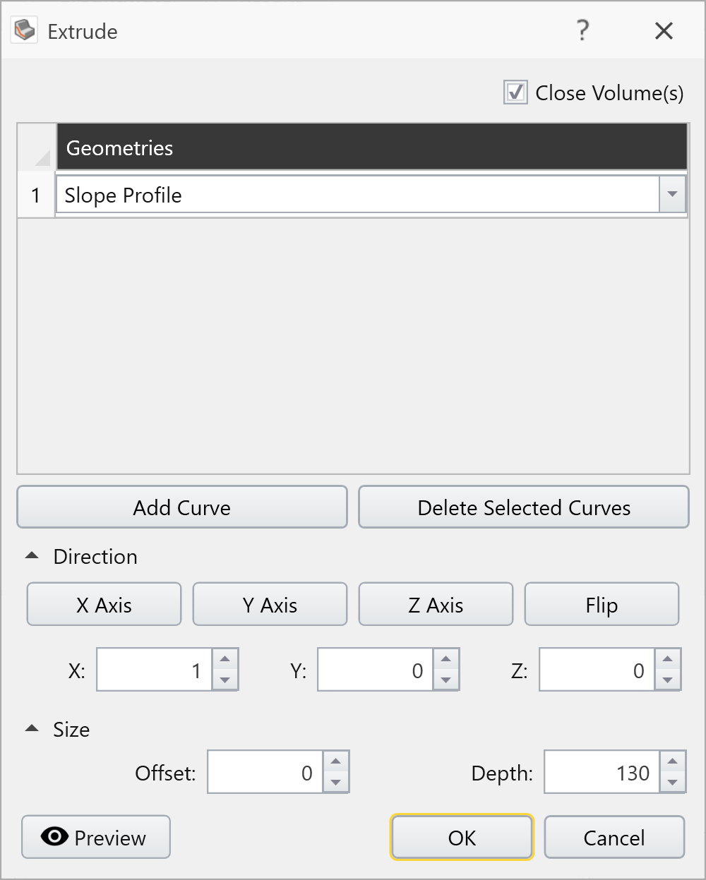
4. Selecting the Preview button will update the viewports with the new geometry. Check to see if the extrusion parameters are correct. Click OK.

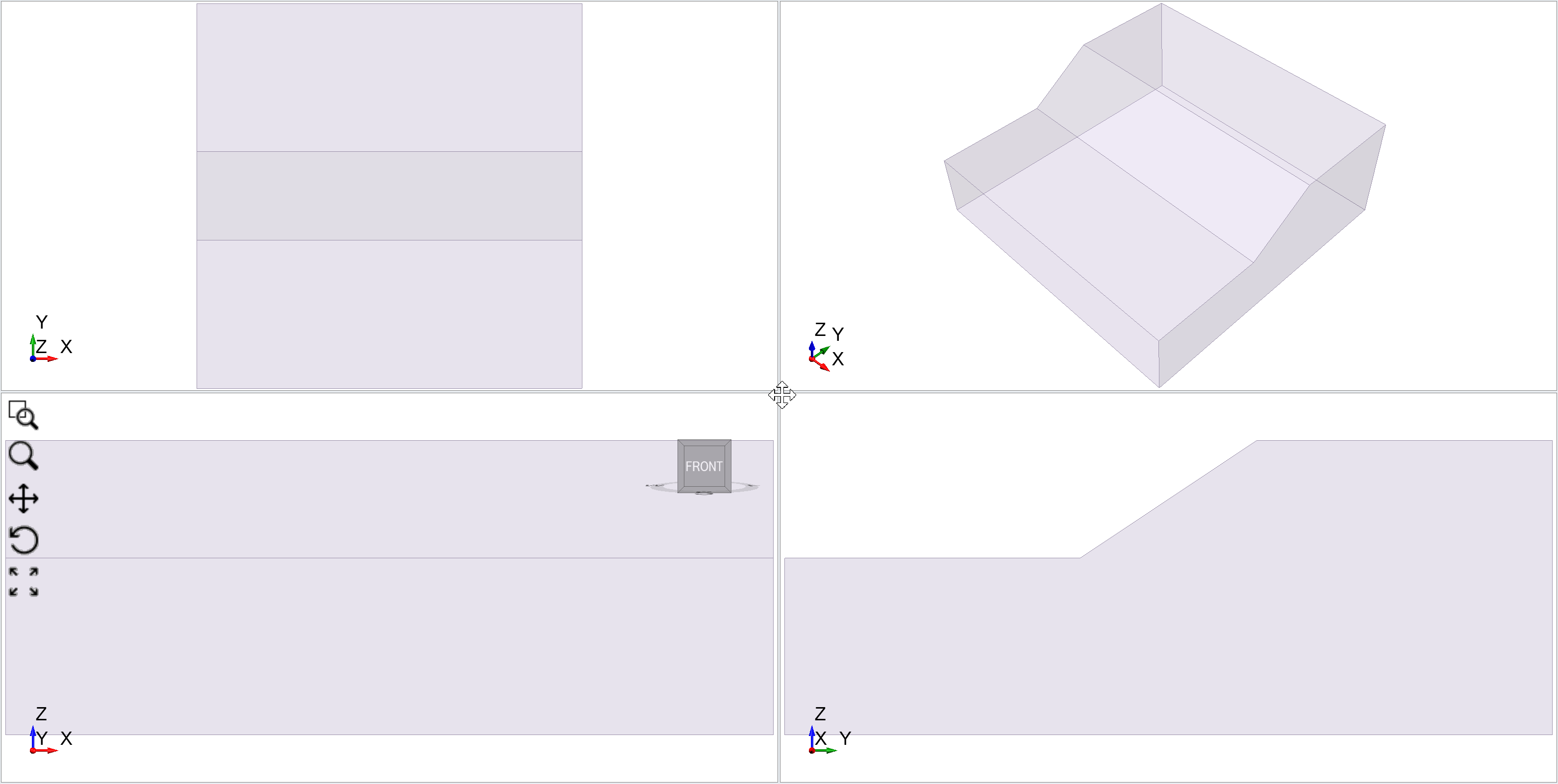
Your viewports should look as follows.

3.4 External Volume

Every Slide3 model must have an External volume defined otherwise the extents of the slope geometry will be unknown.

1. In the Visibility pane select the Slope Profile_extruded entity we have just created.
2. Select: Geometry > Set as External.

The extruded slope volume is now defined as the External volume (also shown with a Lock icon).

3.5 Symmetry

There's one most step we need to take regarding the geometry. To ensure symmetric results for 2D extruded models, you can use the Symmetry option in Project Settings. If the Symmetric Model checkbox is selected, the search results and global minimum slip surface will be constrained to be symmetric along a user-defined vertical plane of symmetry.

1. Select Analysis > Project Settings   and select the Symmetry tab
2. Select the Symmetric Model checkbox
3. Enter the following XY values (65,0) for Point1, (65, 130) for Point 2 and select OK.
   
   
   
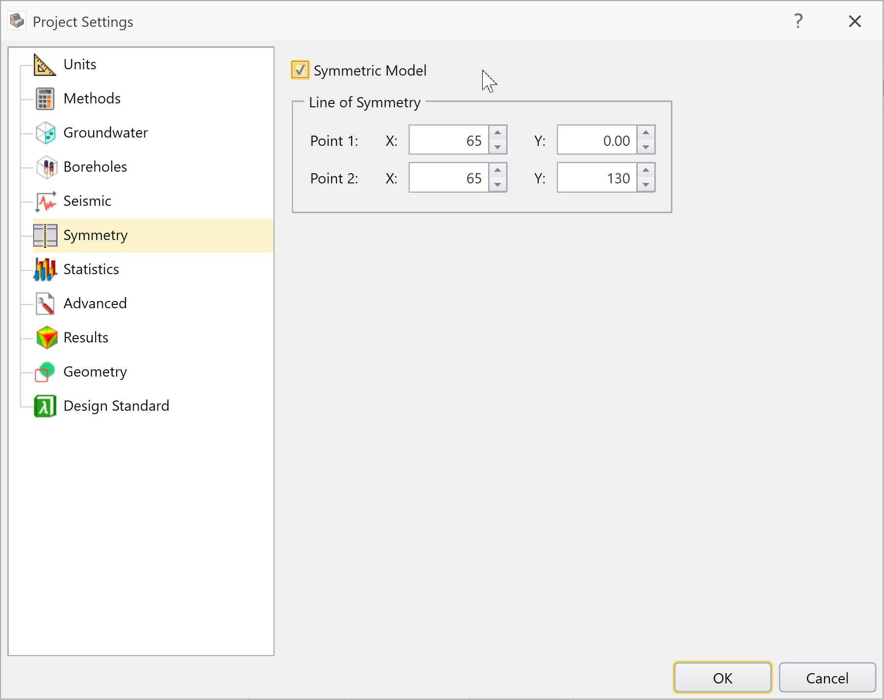
   This defines a line of symmetry in the XY plane down the center of the model.
   Press F2 to Zoom All. If you select the Slip Surfaces tab, you will see the line of symmetry displayed as a white dotted line above the model in the top and perspective views.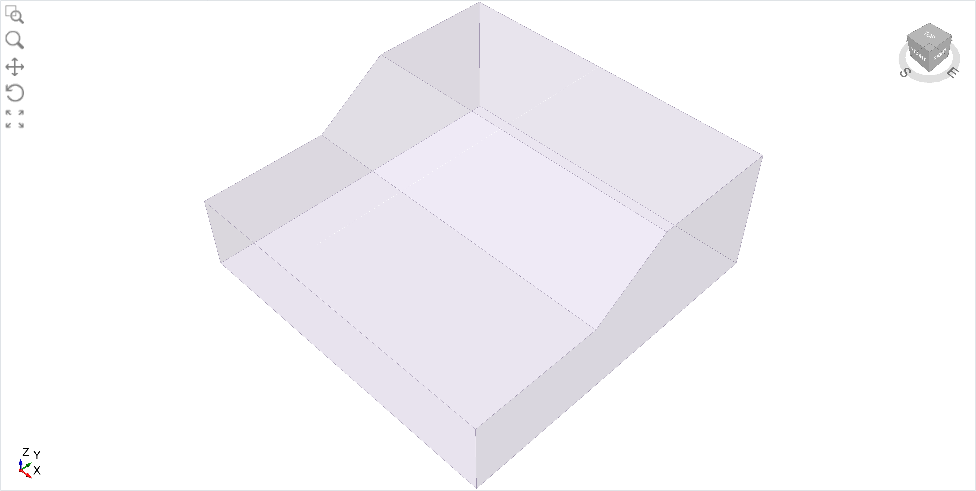
   
   

Line of symmetry displayed (white dotted line).

4.0 Define Materials

For the purposes of this tutorial our model will be composed of only one type of material (clay).

1. Select Materials > Define Materials
2. Enter the following for Material 1:
• Name = Clay,
• Unit Weight = 19,
• Cohesion = 5 kPa, and
• Phi = 30°



3. Click OK.

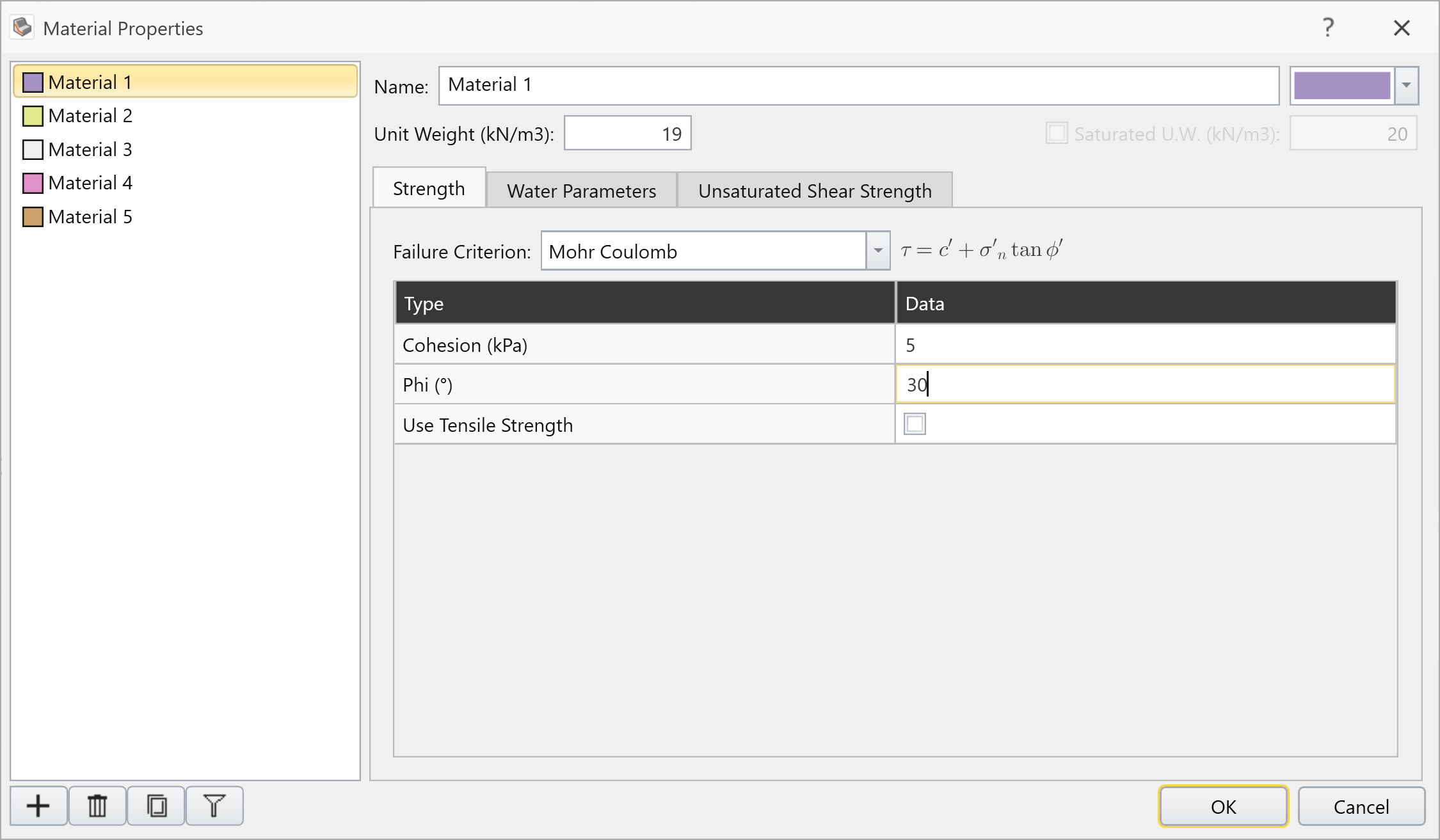
By default, Material 1 is automatically assigned to all volumes within the External volume.

5.0 Slip Surfaces

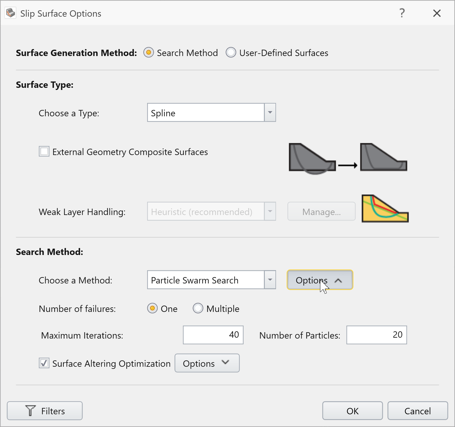
We will use following settings in the Slip Surface dialog:

1. Select Surfaces > Slip Surface Options
   
2. Select:

• Surface Generation Method = Search Method
• Surface Type = Spline
• External Geometry Composite Surfaces = OFF
• Search Method = Particle Swarm Search
• Surface Altering Optimization = ON
  
  

6.0 Compute

Save the model before computing. Then, run the analysis.

1. Select Analysis > Compute

Compute should only take 2 or 3 minutes for this simple model.

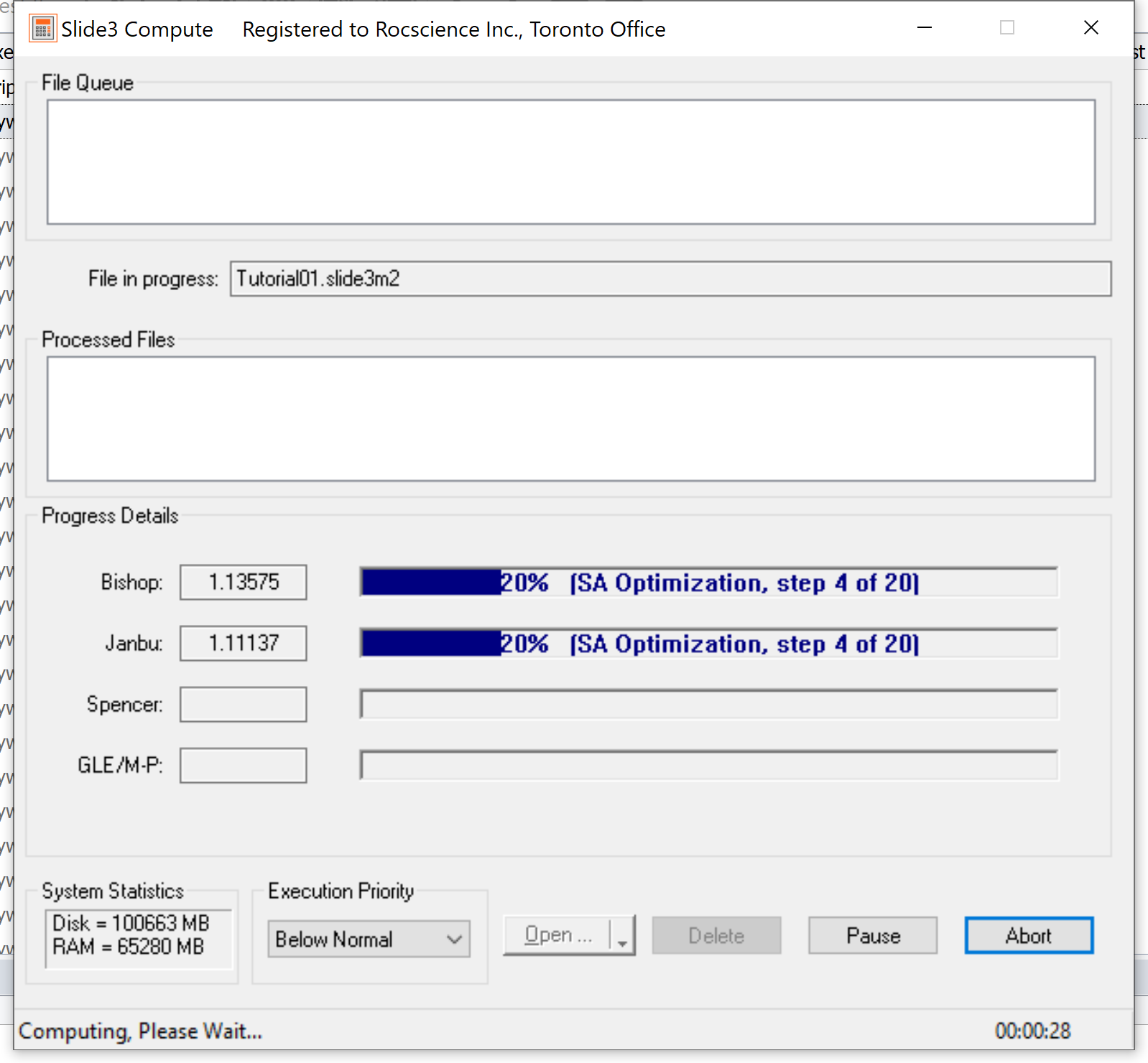
When the Compute dialog closes you can view the Results.

7.0 Results

1. To view the results, select the Results Workflow tab

The Global Minimum slip surface for the Bishop analysis will be displayed. The safety factor (FOS) for the Bishop surface is around 1.1.

2. To view data contours on the slip surface select the Show Contours on the toolbar button .

By default you will see Base Normal Stress contours (i.e. the normal stress on the base of the columns).

3. To view the Janbu safety factor, select Janbu from the Method dropdown in the toolbar. The Janbu safety factor is about 1.1.

To view other data contours, you can select different options from the Data dropdown menu in the toolbar (e.g. Shear Stress).

8.0 Add Water Table

1. Select the Geometry Workflow tab

2. Select Geometry > Polyline Tools > Draw Polyline
   
3. Select the YZ Plane Orientation option.
   
4. Select the Edit Table button in the Coordinate Input area of the sidebar.
   
   
   
5. In the Edit Polyline dialog, select the Append Rows button , add 4 rows and click OK. Enter the following coordinates in the dialog and select OK.
   
   

U	V
5	30
50	30
85	40
135	40

Or,

You can import csv files by selecting Import , and open the file 'Watertable_coordinates.txt' in the tutorial folder. Make sure to choose Space/Tab under delimiter option. Click OK.

6. In the Visibility pane, click on the Polyline entity and re-name it to Water Table.
   
   
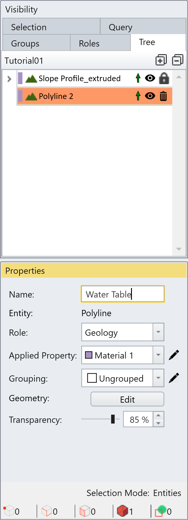
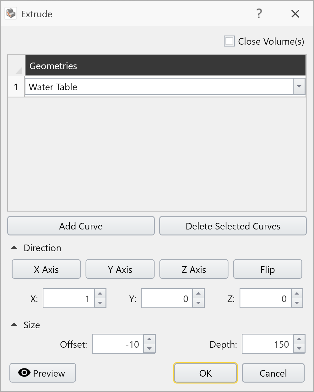
7. Select Water Table entity from the side bar and Geometry > Extrude/Sweep/Loft Tools > Extrude
8. In the Extrude dialog, enter Offset = -10 and Depth = 150. DO NOT select Close Volume(s), as the water table is just a surface. Select Preview to check the input parameters. Select OK.
   
   

the default Groundwater Method can be selected in Project Settings. This determines the initial setting for all materials. The Groundwater Method can also be customized for each individual material in the Define Material Properties dialog.

8.1 Add Water Surface

Although we have added a polyline and extruded a surface, it is not actually a water table yet.

1. Select the Groundwater workflow tab
2. Select 'Water Table_Extruded' entity from the side bar and Groundwater > Add Water Surface
   
3. Select OK to define the surface as a Water Table.
   
   
   
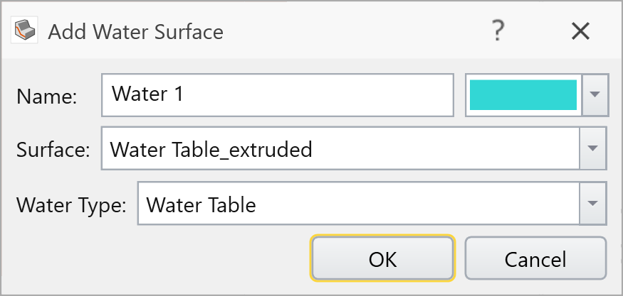
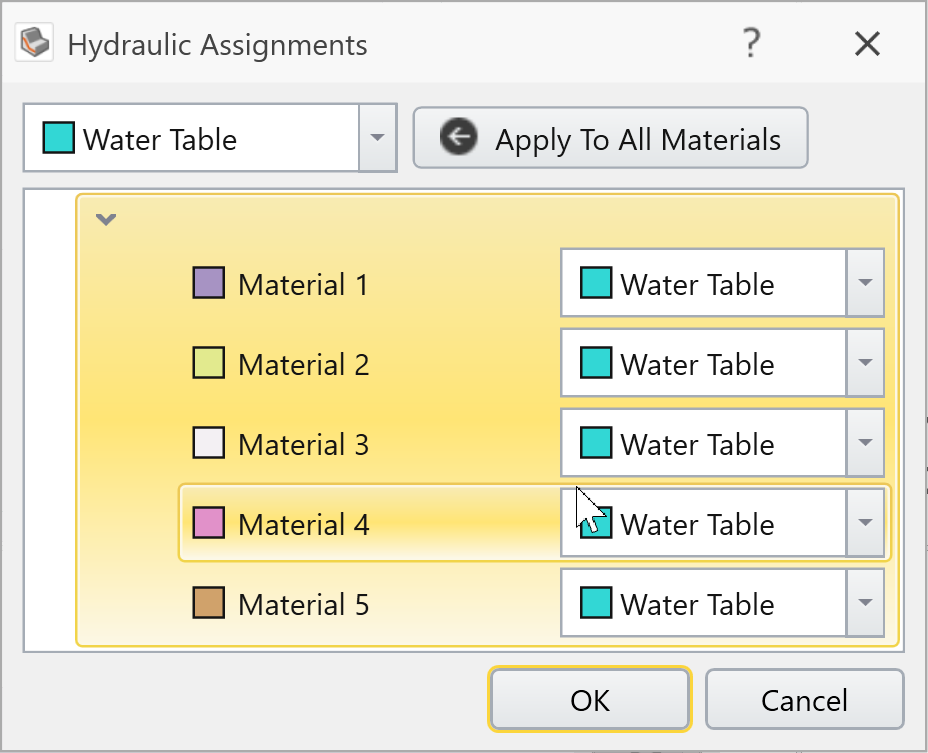
4. You will then see the Hydraulic Assignments dialog. Select OK to assign the Water Table to all materials:
   
   
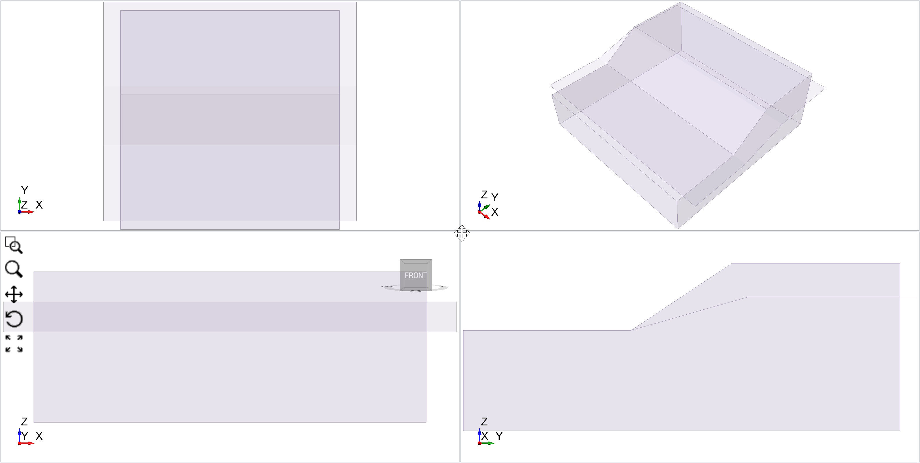
5. The model should look as follows: To double check, slide along Transparency option in Properties pane to see the layers.
   
   
   
   
6. To check the water table assignment, go to the Define Materials dialog and select the Water Parameters tab for Material 1.

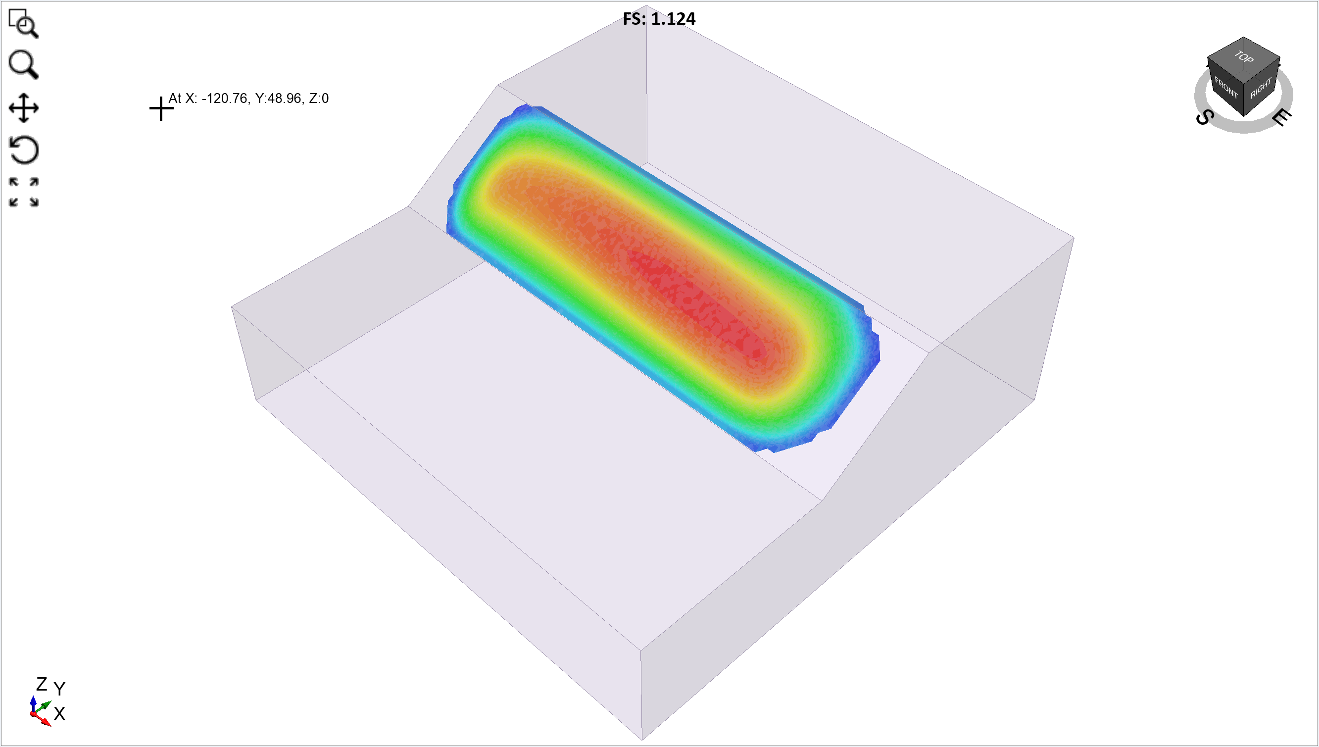
9.0 Results

1. To view the results, select the Results Workflow tab

2. To view data contours on the slip surface select the Show Contours on the toolbar button.

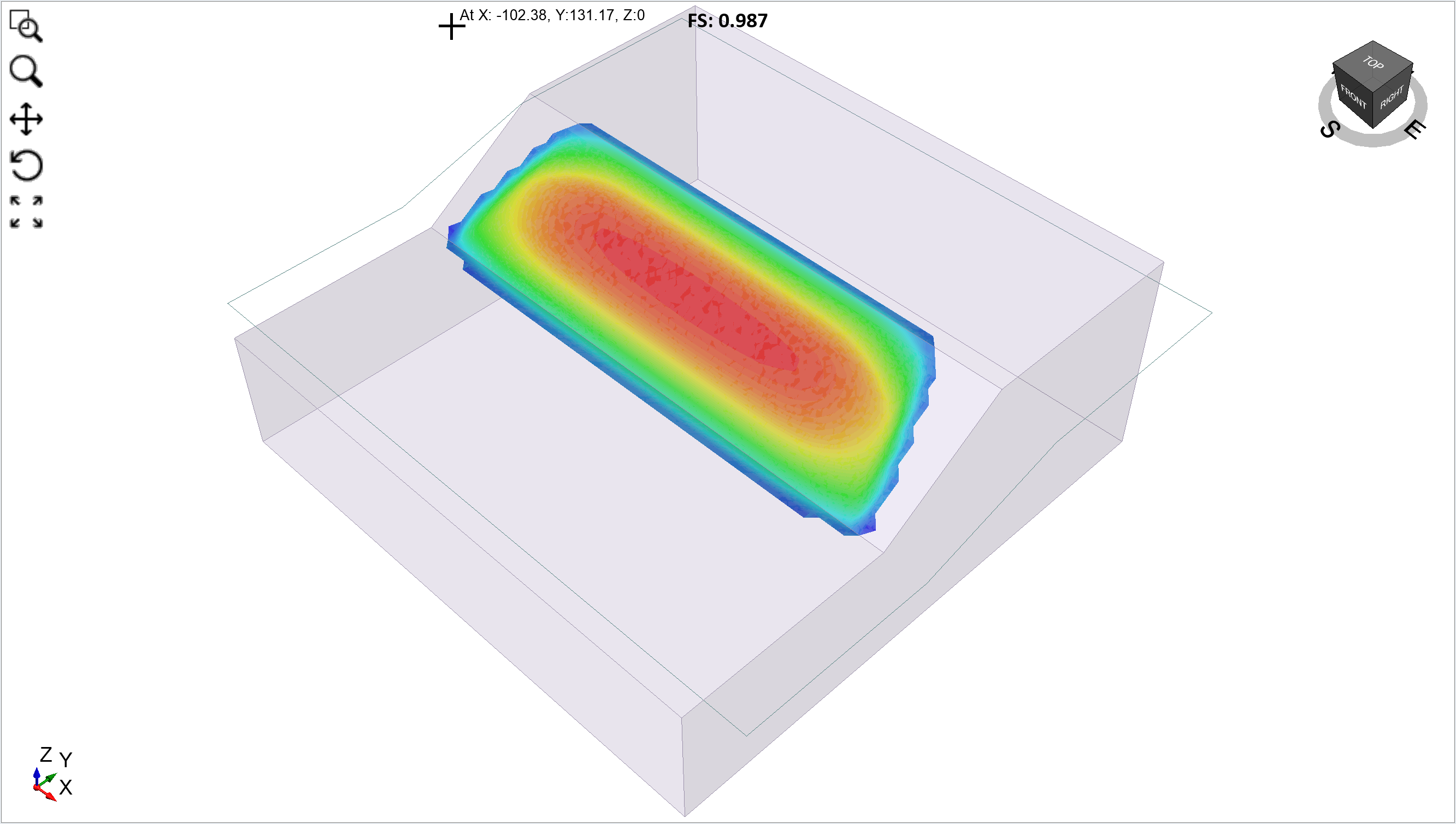
The Bishop safety factor is now below 1.0.