Block Model
1. Introduction
In Slide3, the block model feature allows you to create a model with a rectangular grid of blocks in 3D space, with each block containing its associated material properties.
To begin the tutorial, open the Block Model - starting file.slide3m2 tutorial file from the Tutorial folder.
2. Define Surface Options
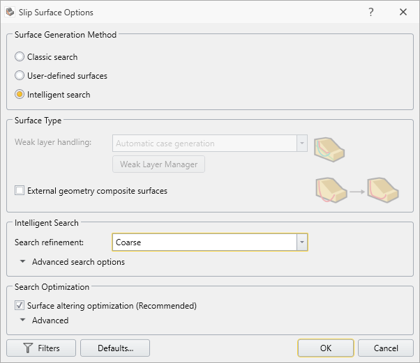
To start, we will update the surface options to use Slide3’s Intelligent Search.
- Select Surfaces > Slip Surface Options.
- Change the Surface Generation Method from Classic Search to Intelligent Search.
- Change the Search refinement from Moderate to Coarse.
3. Block model import
Next we will import the block data.
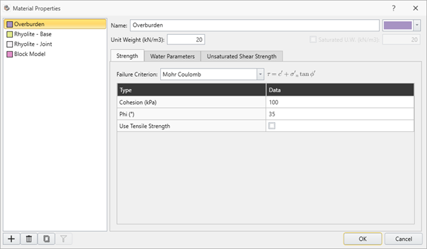
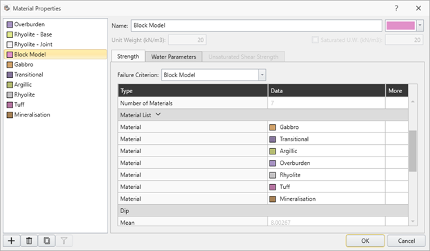
- Select Materials > Define Materials.
- Notice that four materials have been pre-defined. Overburden is a Mohr Coulomb material, whereas the Rhyolite materials are Generalized Hoek-Brown.
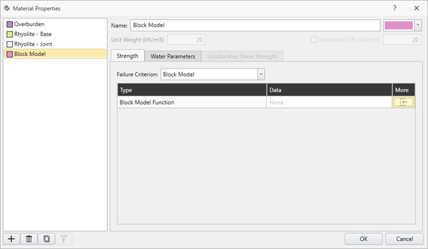
- Click on the Block Model material.
- Set the Failure Criterion to Block Model.
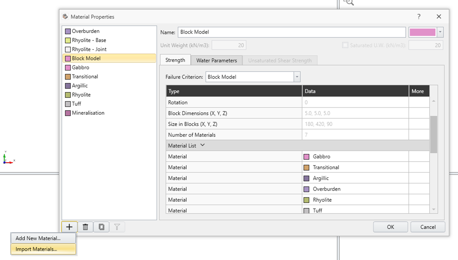
- Then, select the Import icon to import the block model.
- Import the Block Model.csv file that is in the “Block model - starting file” tutorial folder.Slide3 currently only supports block models with all blocks having the same size. Sub-celled models, or models that contain blocks of differing sizes, are not currently supported.Now we must select which material properties we want to vary at the block level. If we choose GSI, for example, we can have a different GSI value assigned to each block in the same material. In our case we will have a block-level Dip, Dip Direction and GSI. Note that defining block-level data is entirely optional.
- Check the Dip, Dip Direction, and GSI boxes.
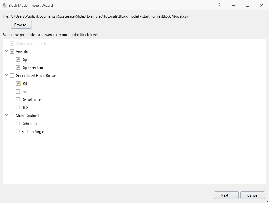
- Click Next.
-
On the left-hand side, set the column number for each parameter. In this case your final column numbers should be as follows. Make sure to set the Start Row to 2 so that the header text is not included. The top pane is the raw csv file. The bottom pane displays the columns you have selected for each parameter.
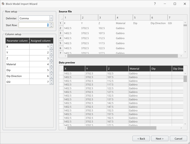
- Notice that not all materials have Dip, Dip Direction, and GSI defined. Only the materials that will use it need to have it defined as will be shown later in the tutorial. Click Next. It may take a few seconds for the block model to be read.
-
Now, we need to input critical information that will define the block model (block size, number of blocks, etc.). First, we will let Slide3 estimate these values automatically. Click the Estimate button.
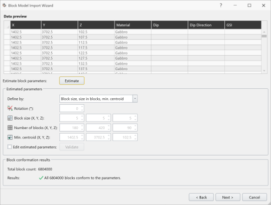
We can see each block is 5 by 5 by 5 units, and other details. If you need to modify the values for any reason, you can always check the “Edit estimated parameters” box to modify them, and then click the Validate button when done. The Define by drop down allows you to select from several different ways to define the block model, common to the output from other programs:- Block Size, Size in Blocks, Minimum Corner
- Block Size, Size in Blocks, Minimum Centroid
- Block Size, Minimum Corner, Maximum Corner
- Block Size, Minimum Centroid, Maximum Centroid
- In this case we are happy with the values so will not edit them. Click Next.
- It may take a few seconds for the block model to import. The last step in the wizard will show us any errors or warnings. In this case, it’s letting us know which materials mentioned in the block model file are not defined, and that they will be created with default Generalized Hoek-Brown parameters:
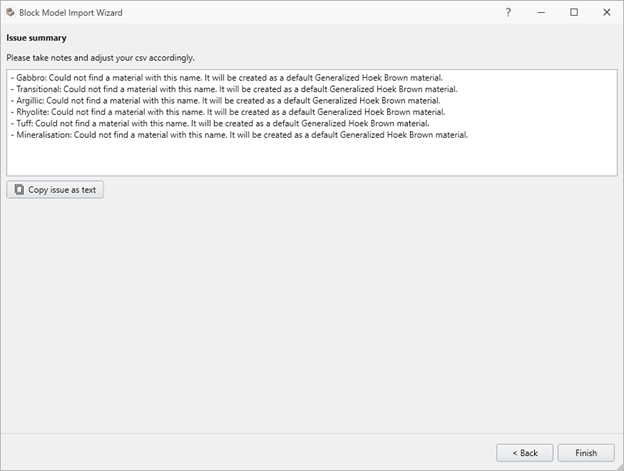
- Click Finish. The block model has been imported and the children materials of the block model have been defined with default parameters. The names of the children materials are taken from the Material column in the block model file.
- Notice that Overburden which we had already defined, was one of the materials listed in the block model file. The Mohr Coulomb properties we had defined for it were not overwritten.
4. Import of material properties
Click through the materials (Gabbro, Transitional, etc.) and you will see they are all defined with default Generalized Hoek-Brown materials. The next step will be importing the material properties of these materials.
Click on the plus button on the bottom left of the dialog and select Import Materials.
We need to import Generalized Hoek-Brown materials. We’ll do this as follows:
- Set the Material Strength Type to Generalized Hoek-Brown. Check the Import Unit Weight box.
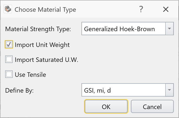
- Click OK.
- Select the Material Properties.csv file from the tutorial folder and click Open.
- Match up the columns to the Generalized Hoek-Brown properties on the left-hand side. You should have the following:
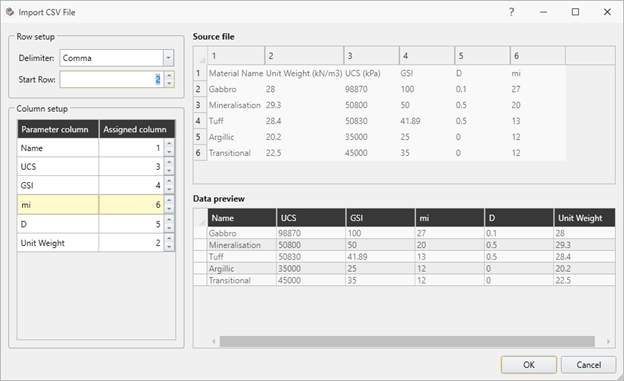
- Click OK.
-
You will see a message letting you know that five material names already exist in Slide3 and asking you if you would like to overwrite them. Click Select all to overwrite all of them with the imported properties.
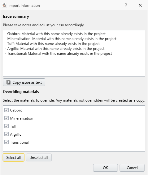
- Click OK.
5. Block-level data
Block-level data is data that differs at the block-level within the same material. We have two materials with block-level data.
Rhyolite is an anisotropic material that will read block-level Dip and Dip Direction from the block file:
- Click on Rhyolite and set the Failure Criterion to Generalized Anisotropic. Click the pencil button.
- Set the Base Material to Rhyolite – Base.
- Set the joint material to Rhyolite – Joint.
- For the Dip and Dip Direction, we will use the block-level data imported with the block data file. Click the Select hyperlink in the Block Data column.
- Check both Dip and Dip Direction, to have them read from the block data file:
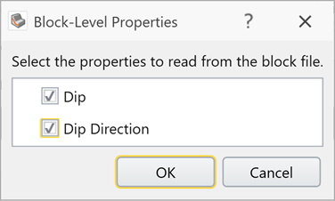
- Click OK.
- Finally, set A=5 and B=10.
- Notice that we can now see some summary statistics bout the Dip data and Dip Direction data in the cells:
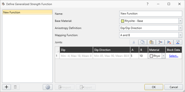
Different blocks within the Rhyolite materials will have different dip and dip direction values as defined in the block data file. - Click OK in the Generalized Strength Function dialog.
Finally, we want the Mineralisation material to read the GSI from the block file:
- Click on Mineralisation material. Notice that in the Block Data column, only GSI is enabled, since that is one of the block-level options we selected.
- Check the GSI box and notice the GSI summary statistics will be displayed:
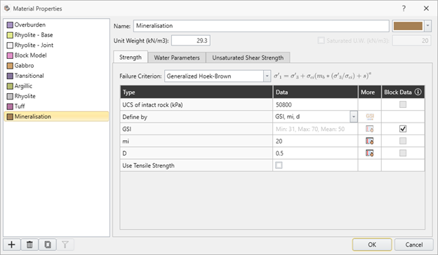
- Click OK in the Material Properties dialog.
We have now defined all the materials.
6. Importing the geometry
Now that the block data is imported, we will import a pit shell to create the geometry:
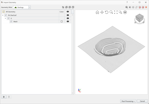
- Select File > Import > Import Geometry.
- Select the Pit Shell.dxf file in the tutorial folder.
- Click Open.
- Check All Geometry and click Post-Processing.
- It is always good practice to simplify geometry and repair defects. In this case we are confident in the quality and will skip these steps. Click Done.
The pit shell will look as follows: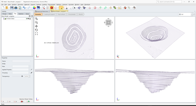
- We’re going to make this into a volume. Select the pit shell in the tree.
- Select Geometry > Create External from Surface.
-
Set the Bottom Elevation to 100.
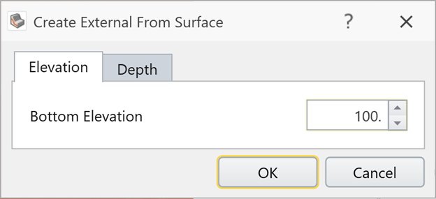
- Click OK.
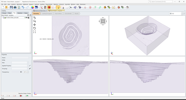
Now we’re going to assign the Block Model material to the external. When we do this, two things will happen:
- A Block Model node will be added to the tree. This will represent the entire block model imported from the file.
- The block model will be projected onto our external.
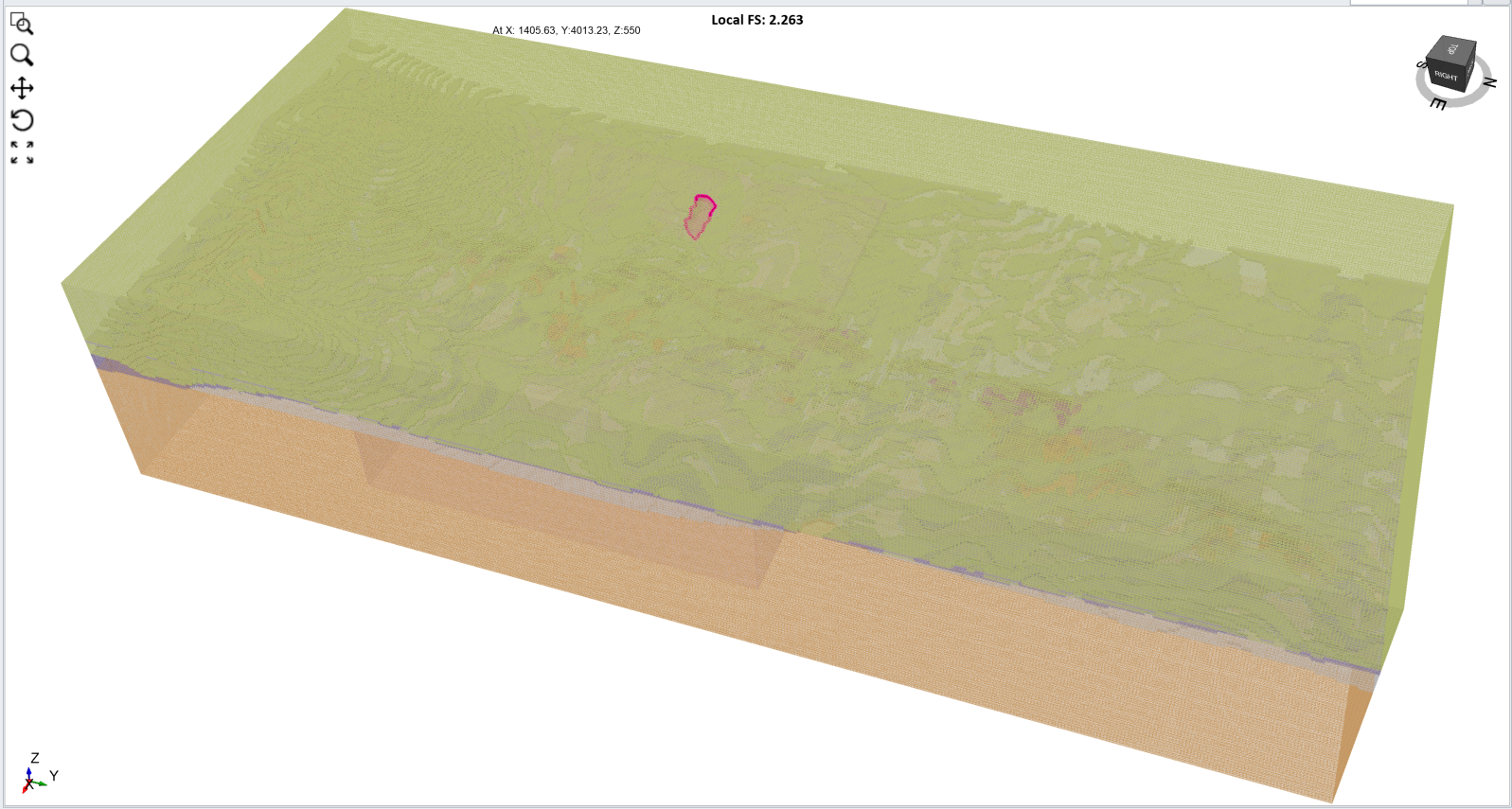
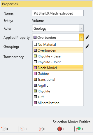
Click on the external in the tree and set the Applied Property to Block Model.
Turn off the visibility of the Block Model item in the tree to see the block model projected onto the external (we can set the transparency to 0 for better visibility):
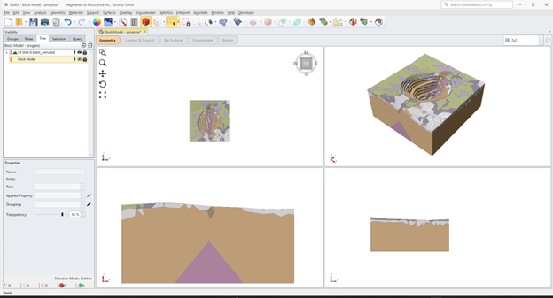
Now we are ready to compute.
7. Compute
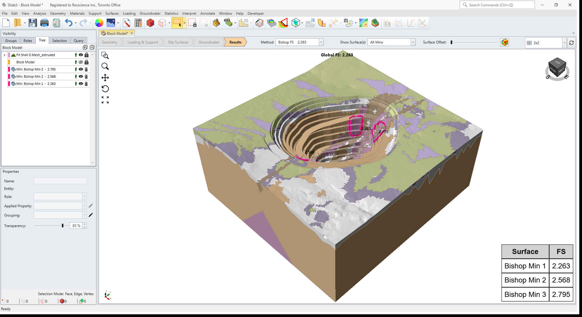
Select Analysis > Compute.
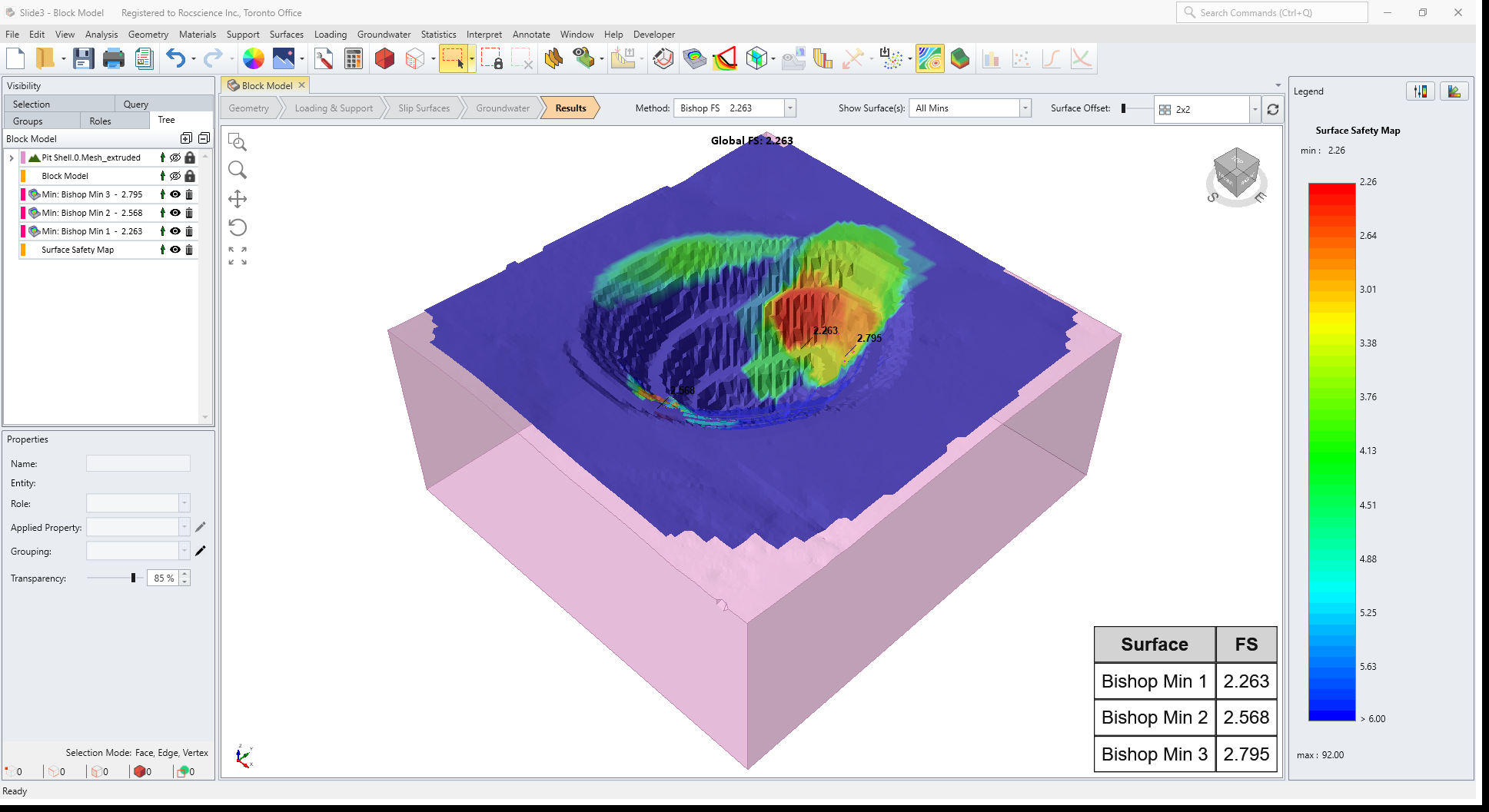
Once done, click on the Results tab. Turn on visibility of the external, and turn off the visibility of the ROI Surface Safety Map.
Now click on Interpret > Add Surface Safety Map to get a better visual of the weak regions.
Finally, you can select Interpret > Column Data Viewer to view detailed analysis results for individual columns in a sliding mass.
8. Export to Slide2
Select Interpret > Create 2D Sections through Global Minimums.
We can see that a section is automatically added through the center of the global minimum result, in the direction of failure. For this tutorial, we only want to focus on the surface with the lowest factor of safety result, so we will delete the first two and only keep Section 3: Bishop Min 1. In this case we are interested in the right side of the slope, so we will change the Failure Direction from Auto to Right to Left.
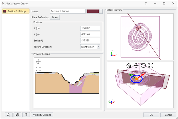
Click OK to exit the Slide2 Section Creator dialog.
Now we will view the projection on the section.
Turn off the visibility of the Pit Shell and results so that the only geometry visible is Section 3 : Bishop Min 1.
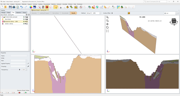
Make sure that Section 3 : Bishop Min 1 is selected and then click Open.
Slide2 will open with our newly created Slide2 file.
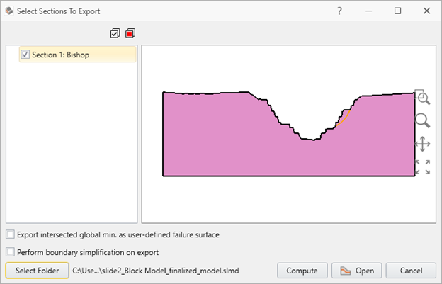
We can see there are a lot of vertices on the model, which will impact the compute time. We will do a boundary simplification on the model.
Go to Boundaries > Simplify Boundary… and using the selection tool, drag to select the entire model.
We will change the Percentage of original vertices value to 30 in the Simplify Boundary dialog. Press OK.
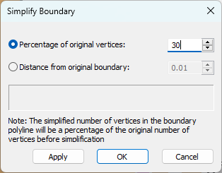
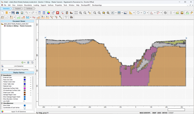
Save your changes.
Now we will look at the Material Properties that got exported from Slide3.
Select Properties > Define Materials.
Select the Mineralisation material. Like in Slide3, we can see that the GSI parameter is using the block data as expected, and that we have the option to turn it off. The other parameters such as UCS, mi, and D cannot be activated because these parameters were not imported with the block model.
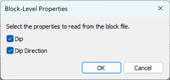
Select the Rhyolite material. Click on the edit button in the grid to view and/or edit the Generalized Anisotropic function. We can see that the Dip and Dip Direction are using the block data values as expected. Click Select… under the Block Data column. We can see in this Block-Level Properties dialog that we have the option of whether to use these Dip and Dip Direction properties from the block model, like in Slide3. Press OK
Press Cancel in the Define Generalized Anisotropic Strength Function dialog and then Cancel in the Define Material Properties dialog.
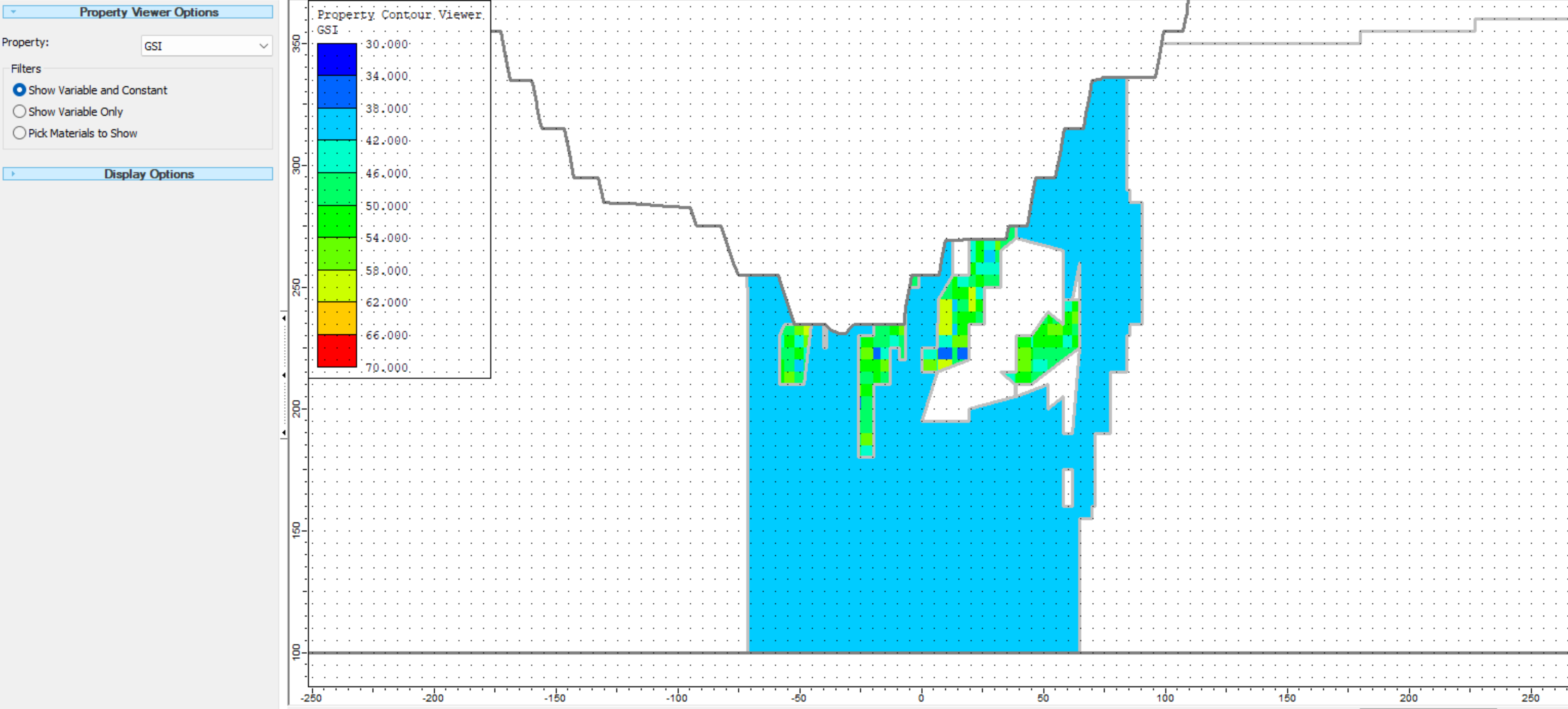
Now we will view the block-level properties in the Property Viewer.
Select Analysis > Property Viewer.
Under Property Viewer Options, select GSI.
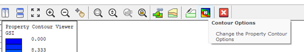
We can now see that Mineralisation material has slight variations in colour where the blocks have different values. To make the contrast more noticeable, we will edit our Contour Options.
In the toolbar, select the Contour Options.
Change the Contour Range to Custom Range, and we will set the Min to 30 and the Max to 70.
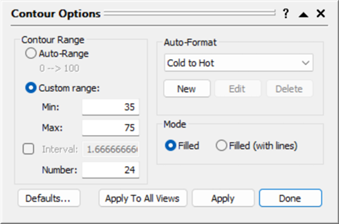
Press Apply.
Now we can see much more clearly what the value is in each block of the Mineralisation material.
By zooming in and hovering your mouse over each block, you will be able to see the exact GSI value of the block.
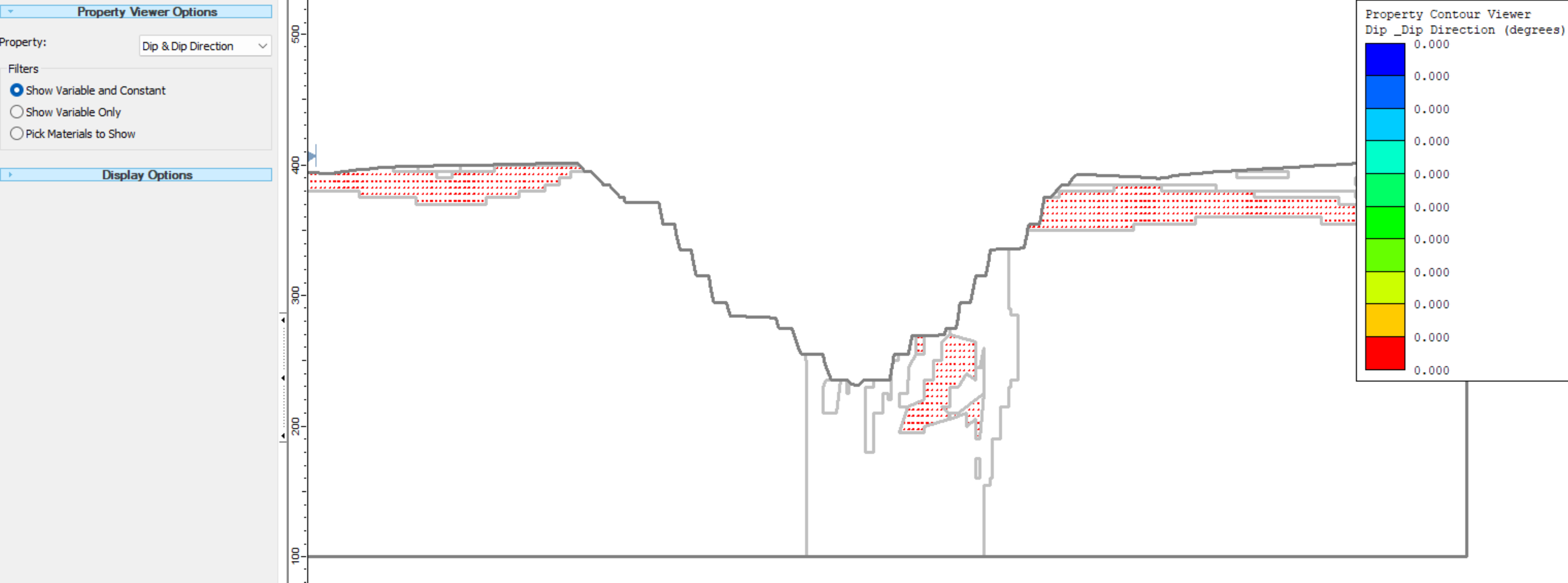
Now we will look at the Dip and Dip Direction for the Rhyolite materials. In the Property Viewer Options, select the Dip & Dip Direction property.
We can now see the red lines that are drawn on the model, and if we zoom in, we can see that they represent the Dip and Dip Direction per block.
Finally, go back to the Slide3 model, and select Analysis > Slide2 Integration > Slide2 Recompute.
View the results of the model with the results of the section: