Effects of Thermosyphon on Shallow Foundation
1.0 Introduction
1.1 Problem description
This problem addresses the use of RS2 to simulate the effects of thermosyphon on a shallow foundation in a cold climate to prevent the thawing of the permafrost. A concrete structure will be constructed on a shallow foundation of clay. Thermosyphon will be installed one year in advance of building the structure. The concrete structure will be supported by insulated joints.
The analysis is taken over a period of two years, starting from thermosyphon installation, one year before the concrete structure construction. The tutorial demonstrates the thermosyphon modelling methods with RS2 thermal module by:
- Set up initial temperature (Stage 1) - Section 2.6
- Assign thermal boundary conditions to the external boundaries before the building construction (Stage 2-12), such as flux constant, flux climate boundary conditions - Section 2.7.3
- Install thermosyphon (Stage 2-24) - Section 2.7.1
- Assign thermal boundary conditions to the model after the building construction (Stage 13-24), such as insulation, temperature, and flux climate boundary conditions. - Section 2.7.2 and 2.7.3
With the RS2 Thermal module, thermal properties are applied to the model in various aspects including materials, initial model temperature, external geometry boundary conditions, joint boundary conditions, and thermosyphon, to perform a thorough thermal analysis.
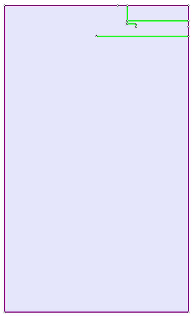
1.2 Initial model
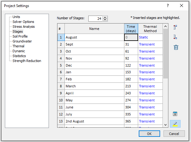
In the starting model file, the stage numbers, geometry, boundaries, and field stress have been defined. The time functions for thermal boundary conditions (including air temperature, wind speed, evaporation, solar radiation, albedo, vegetation height, and snow depth) and the temperature grid have been input to save time for the user. 24 stages are used with one-month increments. The thermosyphon will be installed at stage 2 (Sept), and the structure with insulated joints will be built at stage 13 (2nd August).
2.0 Model
- Select: File > Recent Folders > Tutorial Folder
- Open the Effects of thermosyphon on shallow foundation (initial).fez file from the Thermal Analysis folder.
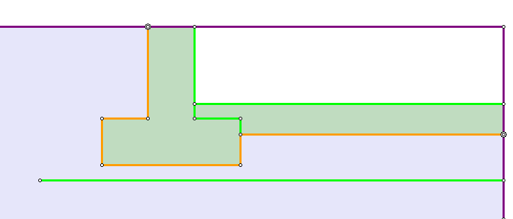
The initial model should look as follows:
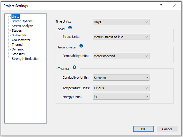
2.1. Project Settings
- Select: Analysis > Project Settings

- Select the Units tab, ensure Time Units = Days.
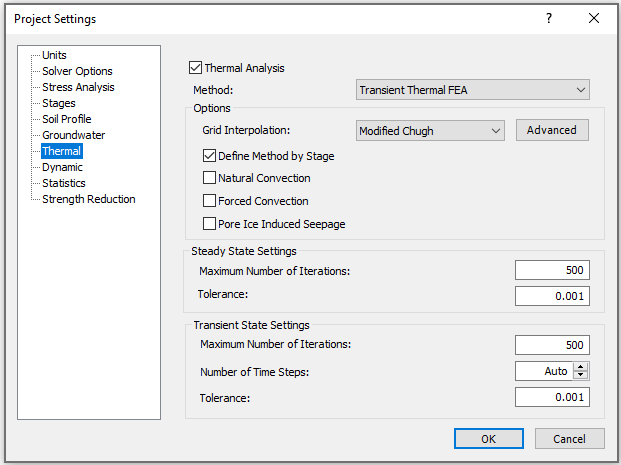
- Select the Thermal tab, and enter the following:
- Set Method = Transient Thermal FEA
- Enable the Define Method by Stage option
- Select the Stages tab. The stage number and name have been defined in advance. Now, we can define the time and thermal method for each stage. The first stage should be changed from steady to static, the rest should be set to transient. The data can be found in an Excel Sheet in the installation folder: C:\Users\Public\Documents\Rocscience\RS2 Examples\tutorials\Thermal Analysis
- Open the file titled “Effects of thermosyphon on shallow foundation” in Excel, select the tab 1. Stages.
- Select the tab Stages in the Project Settings dialog. Copy and paste the time and thermal method from Excel to RS2. Now the model undergoes transient thermal analysis.
- The remaining parameters are left at their default values. Click OK to apply and exit the dialog.
The Thermal tab should look as follows:
The Stages tab should look as follows:
2.2. Material Properties

Define the material properties for clay and concrete, including thermal properties.
- Select: Properties > Define Materials

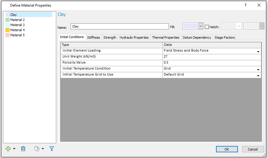
- Select Material 1 from the list in the left of the dialog, change Name = Clay.
- Update the follow material properties for Clay. (Leave all others as the default value.)
Initial Conditions
Type
- Initial Temperature Condition = Grid
- Initial Temperature Grid to Use = Default Grid
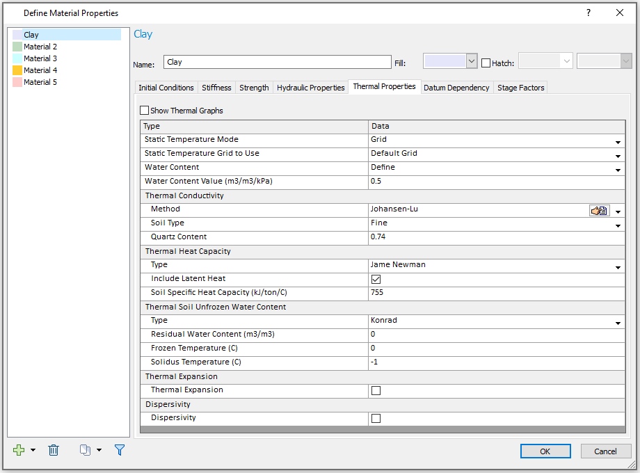
Thermal Properties
Type
- Static Temperature Mode = Grid
- Static Temperature Grid to Use = Default Grid
- Water Content = Define
- Water Content Value (m3/m3/kpa) = 0.5
Thermal Conductivity
- Method = Johansen-Lu
Thermal Heat Capacity
- Type = James Newman
- Include Latent Heat = YES
Thermal Soil Unfrozen Water Content
- Frozen Temperature (C) = 0
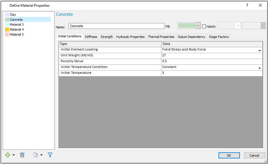
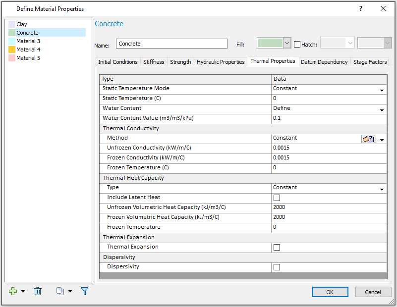
- Select Material 2 from the list in the left of the dialog. Change Name = Concrete.
- Update the following material properties for Concrete. (Leave all others as the Default values.)
Initial Conditions
Type
- Initial Temperature = 3
Thermal Properties
Type
- Water Content = Define
- Water Content Value (m3/m3/kPa) = 0.1
Thermal Conductivity
- Unfrozen Conductivity (kW/m/C) = 0.0015
- Frozen Conductivity (kW/m/C) = 0.0015
Thermal Heat Capacity
- Unfrozen Volumetric Heat Capacity (kJ/m3/C) = 2000
- Frozen Volumetric Heat Capacity (kJ/m3/C) = 2000
- Leave other parameters at their default values. Select OK to apply and close the Define Material Properties dialog.
2.3. Add Joints

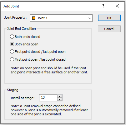
- Select: Boundaries > Add Joint

- In the Add Joint dialog, ensure Joint Property = Joint 1, select Joint End Condition = Both ends open and Install at stage = 13. The dialog should look as follows:
- Click OK to apply and exit the dialog.
- A cross cursor will display to select vertices of the joint boundary. Press “t” on the keyboard to enter a table of coordinates.
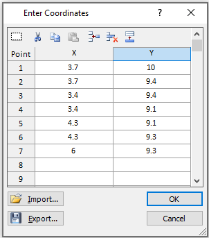
- Enter the coordinates in the table below in the Enter Coordinates dialog that opened. This data can also be found in the “2. Joint boundary coordinates” tab of the “Effects of thermosyphon on shallow foundation” Excel sheet.
- Click OK to apply and close the dialog. Press Enter or select Done from the right click menu to complete selection. Now the joint boundary with both ends open has been added to Stage 13 onwards to support the concrete structure. Click through stages in the model to view the staged installation of joints.
Vertex # |
X |
Y |
|---|---|---|
1 |
3.7 |
10 |
2 |
3.7 |
9.4 |
3 |
3.4 |
9.4 |
4 |
3.4 |
9.1 |
5 |
4.3 |
9.1 |
6 |
4.3 |
9.3 |
7 |
6 |
9.3 |
The Enter Coordinates dialog should look as follows:
2.4. Assign Material
The concrete structure will be built on the 2nd August (stage 13). We will assign concrete to stage 13.
- Select the 2nd August (stage 13) tab in the model.
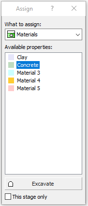
- Select: Properties > Assign Properties

- In the Assign dialog, select Materials and Concrete. The dialog should look as follows:
- Ensure Stage 13 is selected in the model.
- In the model, use the mouse to select the two regions within the joint boundary (orange line). The Concrete property will be assigned.
- In the Assign dialog, select Excavate. Then select the top right region of the model. The model should look as follows:
- Hit the Esc key to exit selection. Close the Assign dialog.
Now the concrete structure with joints supported are installed at stage 13 and onward. Click through stages in the model to view the staged installation of concrete.
2.5. Mesh

- Select: Mesh > Discretize and Mesh

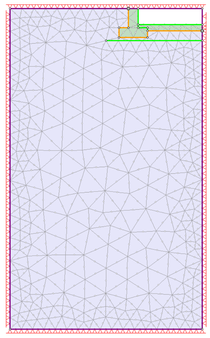
Mesh will be generated, and the model should look as follows:
2.6. Temperature Grid
- Select the Thermal workflow tab

- Select: Thermal > Temperature Grid

The initial temperature distribution can be defined by inputting the temperature grid data into the Temperature Grid dialog. - The data can be found in the “3. Initial Temperature” tab of the “Effects of thermosyphon on shallow foundation” Excel sheet. Copy and paste the x coordinates, y coordinates and temperature to the Temperature Grid dialog.
Now the Temperature Grid dialog should look as follows: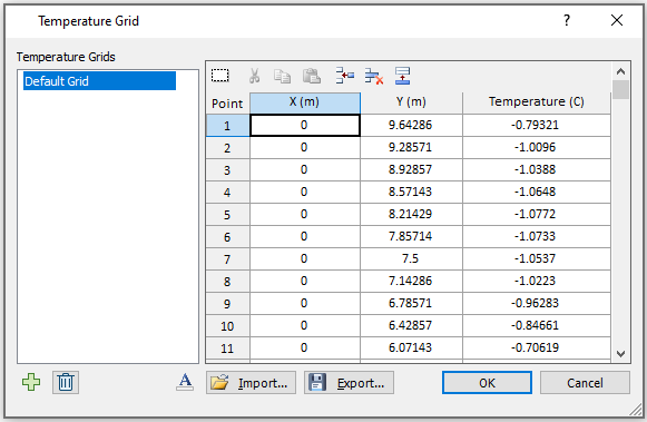
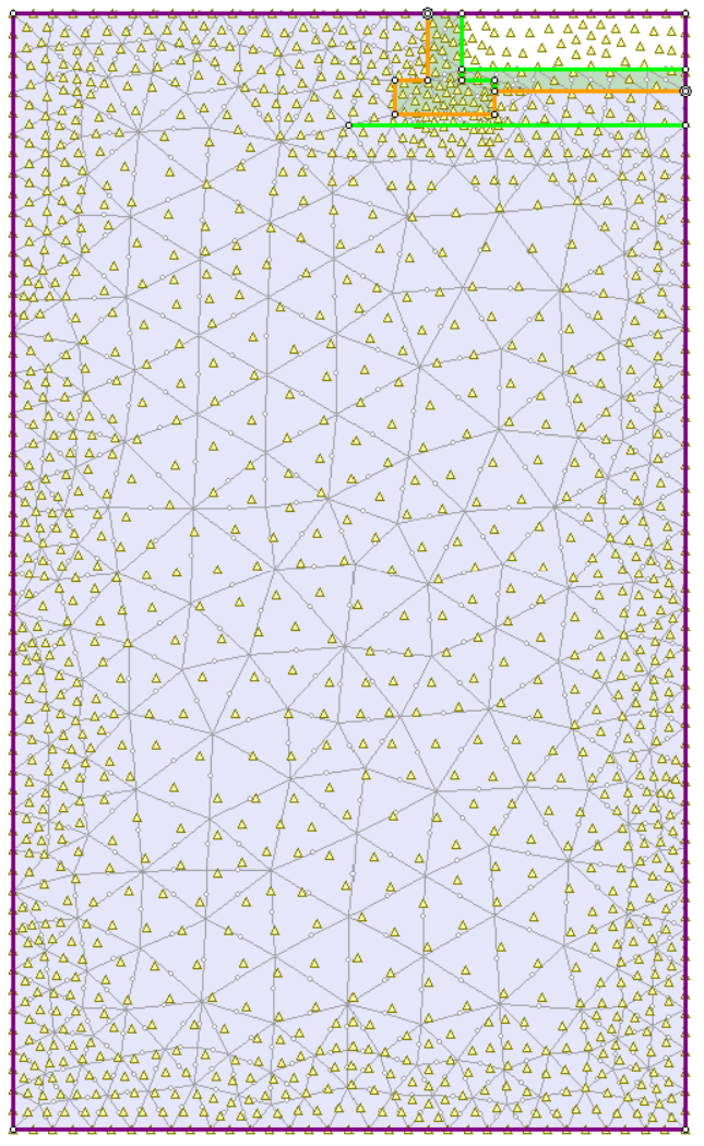
- Click OK to apply and close the dialog. When the temperature grid is applied, the location of each grid point will be marked by a yellow triangle on the model. The model should look as follows:
2.7. Thermal boundary conditions
2.7.1. Thermosyphon boundary condition
A thermosyphon will be added to the model from stage 2 as a thermal boundary condition.
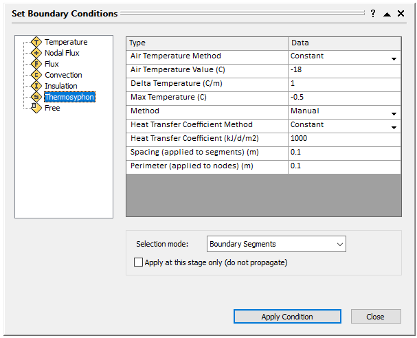
- Select: Thermal > Set Boundary Conditions

- In the Set Boundary Conditions dialog, select Thermosyphon
from the left panel as shown in the screenshot below. Now we can define the properties for the thermosyphon.
- In the main panel, set Air Temperature Method = Time Dependent. Select the “…” button for Air Temperature Function = Temperature 1. In the Define Function dialog, the tabular time function data for Temperature 1 has been defined. The data can be found in the “4. Air Temperature” tab of the “Effects of thermosyphon on shallow foundation”
Excel sheet.
The Define Function dialog should look as follows: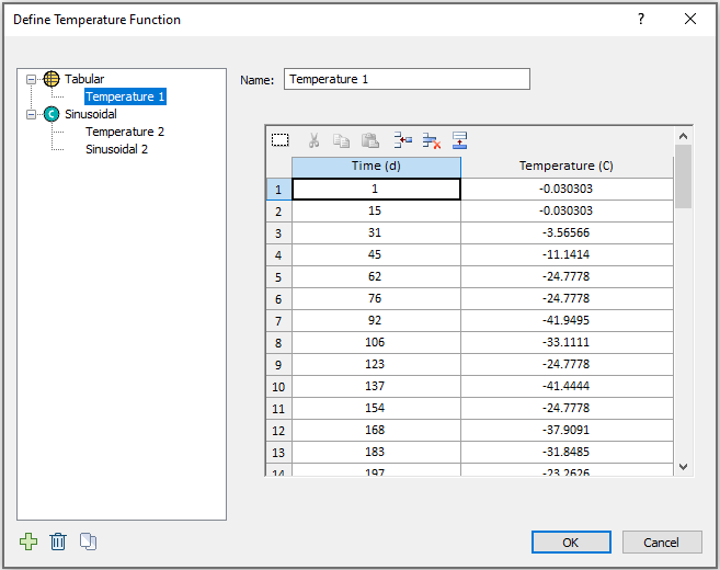
- Click OK to close the dialog.
- In the Set Boundary Conditions dialog, set Method = Zarling and Haynes, Wind Speed Method = Time Dependent. Select the “…” button for Wind Speed Function = Wind 1. In the popped up Define Function dialog, the tabular time function data (Time (d) vs. Wind Speed(m/d)) for Wind 1 has been defined. The data can be found in the “5. Wind Speed” tab of the “Effects of thermosyphon on shallow foundation” Excel Sheet.
The Define Function dialog should look as follows: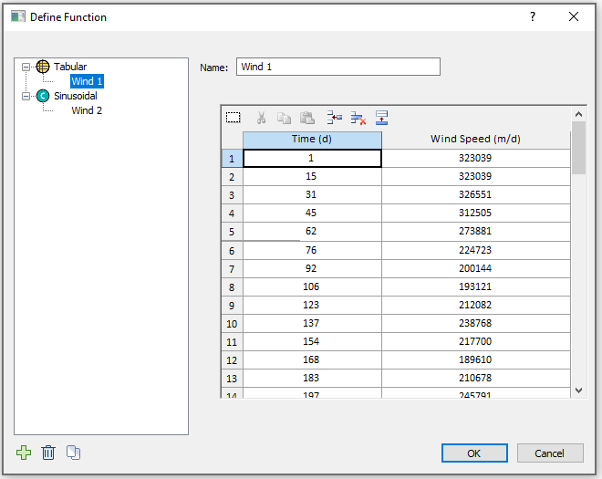
- Click OK to close the dialog.
- In the Set Boundary Conditions dialog, set Spacing (applied to segments) (m) = 2, Evaporator Length (m) = 6.
- Leave the remaining parameters at their default values. The Set Boundary Conditions dialog should look as follows:
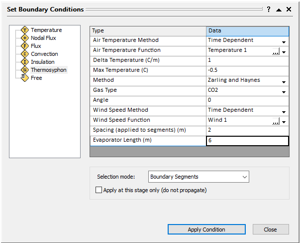
- Ensure Selection mode = Boundary Segments at the bottom of the dialog.
The thermosyphon properties are ready to be applied to the model. To assign the condition, in the modeler: - Select Stage 2. Sept
- Select the material boundary (green line) underneath the joints
- Click Apply Condition in the Set Boundary Conditions dialog
- The thermosyphon boundary condition will be applied to the model as a dashed line with a “S” letter, as follows (b):
- Click Close to exit the Set Boundary Conditions dialog
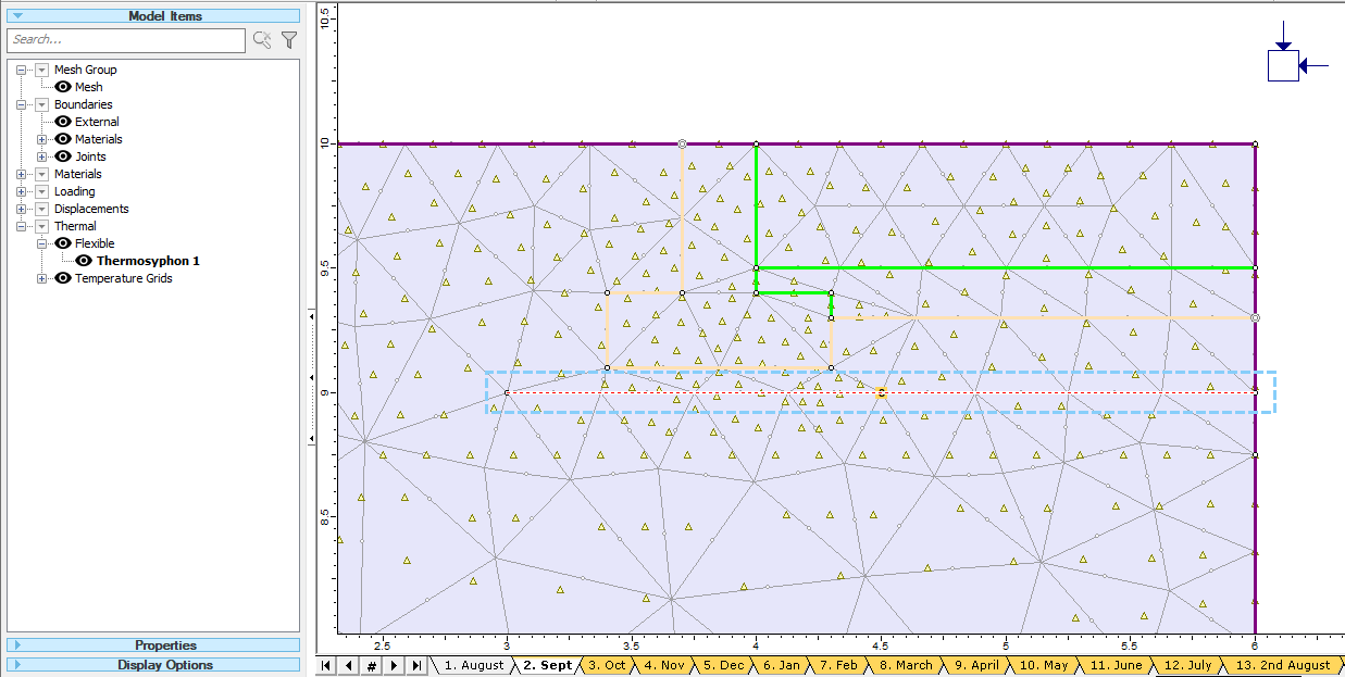
- Under the Visibility Tree, choose Thermal > Flexible >Thermosyphon 1. The thermosyphon will be highlighted in a box. Click through stages to view the staged thermosyphon.
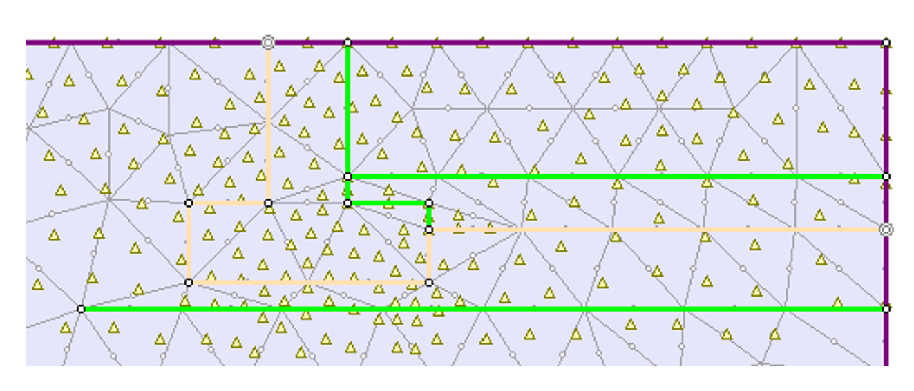 | 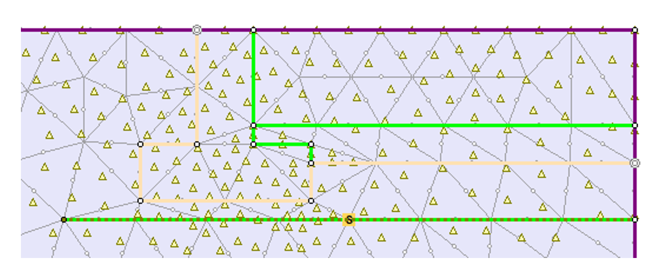 |
| a) Before thermosyphon installation | b) After thermosyphon installation |
Now the thermosyphon has been added with the name “Thermosyphon 1” from Stage 2. Sept to the last stage.
2.7.2. Insulation Boundary Condition
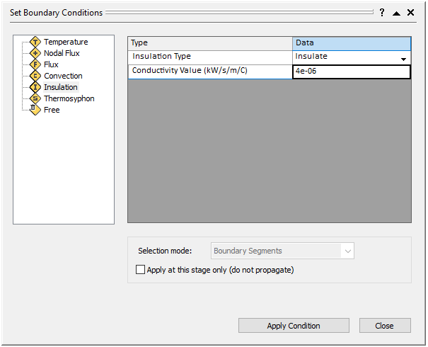
An insulation boundary condition with the conductivity of 4e-06 kW/m/C will be applied to the joint boundary from stage 13 onwards.
- Select: Thermal > Set Boundary Conditions
- In the Set Boundary Conditions dialog, select Insulation from the left panel.
- Set Insulation Type = Insulate, and Conductivity Value (kW/m/C) = 4e-06. The dialog should look as follows:
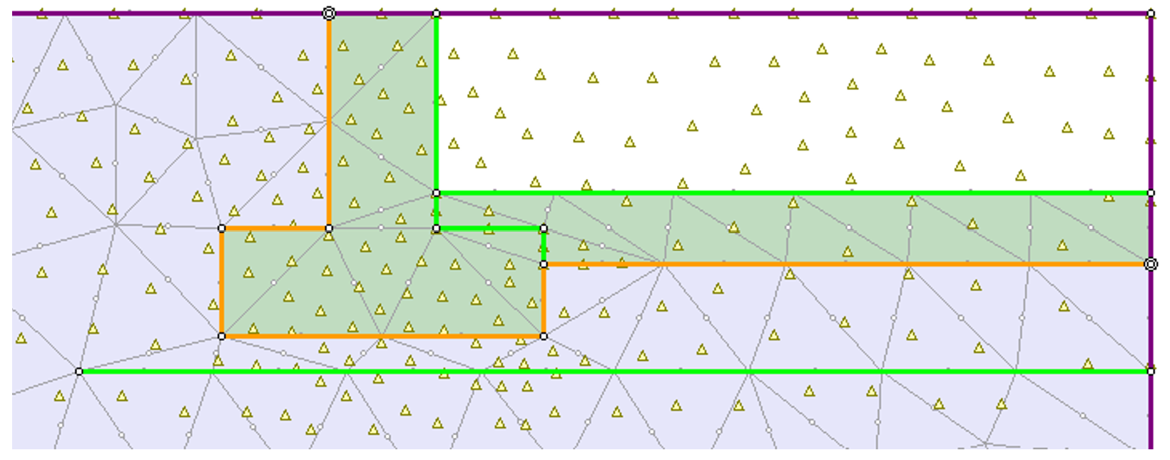
- To assign the condition in the modeler:
- Select Stage 13. 2nd August
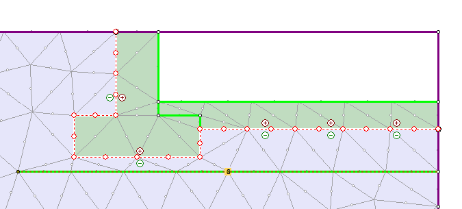
- Select the joint boundary segments (orange line) using the mouse. The current sign convention for the joint boundary bending will display by +/- symbols on either side of the boundary. See the following screenshot:
- Click Apply Condition in the Set Boundary Conditions dialog. The boundary condition will be applied to both sides of the joint boundary.
- The insulation boundary condition will be applied to the model as a dashed line with an “I” letter, as follows (b):
- Click Close to exit the Set Boundary Conditions dialog
- Select Insulation 1 under the Visibility Tree > Thermal > Insulations. The insulation boundary condition will be highlighted in the model. Click through stages to view the staged insulation boundary condition. The model will look as follows:
 | 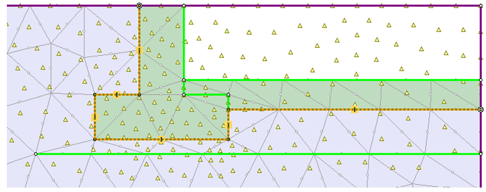 |
| a) Before Insulation Boundary Condition Installation | b) After Insulation Boundary Condition Installation |
Now the insulation boundary condition has been added to the joint boundary with the name “Insulation1” from Stage 13. 2nd August to the last stage.
2.7.3. External Boundary Conditions
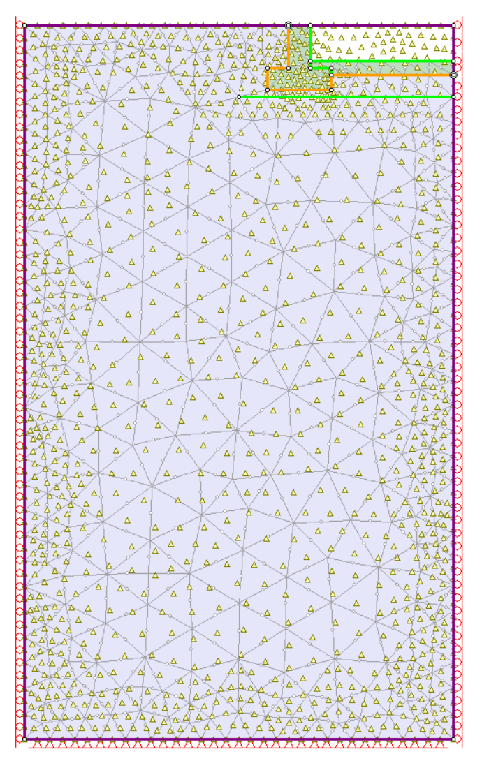
The external boundary segments involving thermal boundary conditions have been divided to five groups as labeled in the picture below. For each group, the thermal boundary conditions throughout the analysis are listed in the table below.
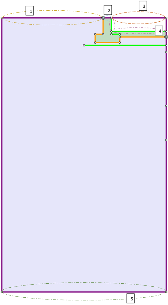
Group |
Note |
Before building the structure |
After building the structure |
||
Stages |
Type of thermal boundary condition |
Stages |
Type of thermal boundary condition |
||
1 |
Top left |
2-12 |
Climate flux |
13-24 |
Climate flux |
2 |
Top middle |
2-12 |
Climate flux |
13-24 |
Constant temperature |
3 |
Top right |
2-12 |
Climate flux |
13-24 |
None |
4 |
Around the building |
2-12 |
None |
13-24 |
Constant temperature |
5 |
Bottom |
2-12 |
Constant flux |
13-24 |
Constant flux |
Therefore, when assigning thermal boundary conditions to a group of segments, make sure the group can be treated as a whole, either until the boundary condition is removed or through the analysis.
To apply these thermal boundary conditions:
- Select: Thermal > Set Boundary Conditions
i. Climate Flux Boundary Condition
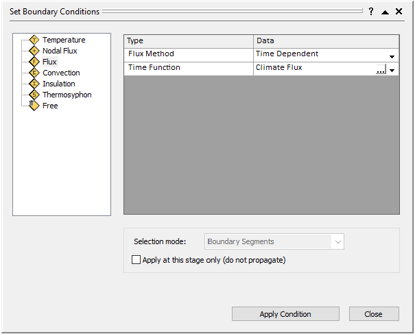
- We start with the climate flux condition for Group 1, 2, and 3. In the Set Boundary Conditions dialog, select Flux from the left panel.
- Change Flux Method = Time Dependent. Select the “…” button beside Flux 1 for Time Function. A Define Function dialog will open.
- Select Flux 3 under the function type Climate from the left panel list. Then, specify the relevant parameters to define a time dependent climate flux condition. The method and equations for the climate flux can be found in the RS2 Thermal Theory Manual.
- In the main panel, Change the Name =Climate Flux, set Total Time = 988, Radiation = Calculate from Solar Radiation, Calculate from Solar Radiation = Define, enable the Define Vegetation option, enable the Define Snow Pack option, and Snow Conductivity = 0.0001. The dialog should look as follows:
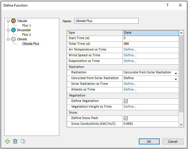
Seven required user defined time functions for Climate Flux have been defined. View the functions by selecting the “Define…” option to the right of each of Air Temperature vs Time, Wind Speed vs Time, Evaporation vs Time, Solar Radiation vs Time, Albedo vs Time, Vegetation Height vs Time, Snow Depth vs Time.
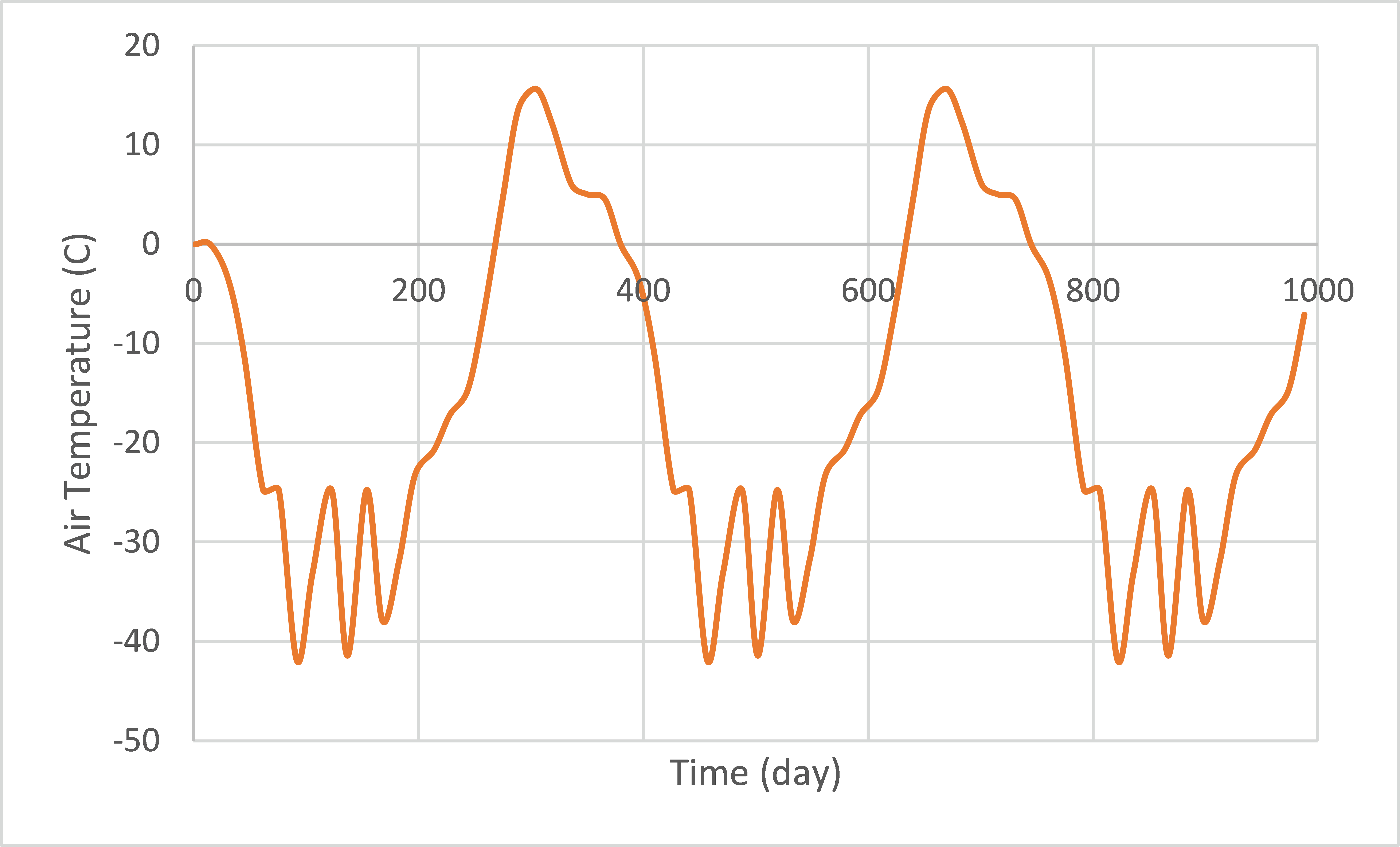
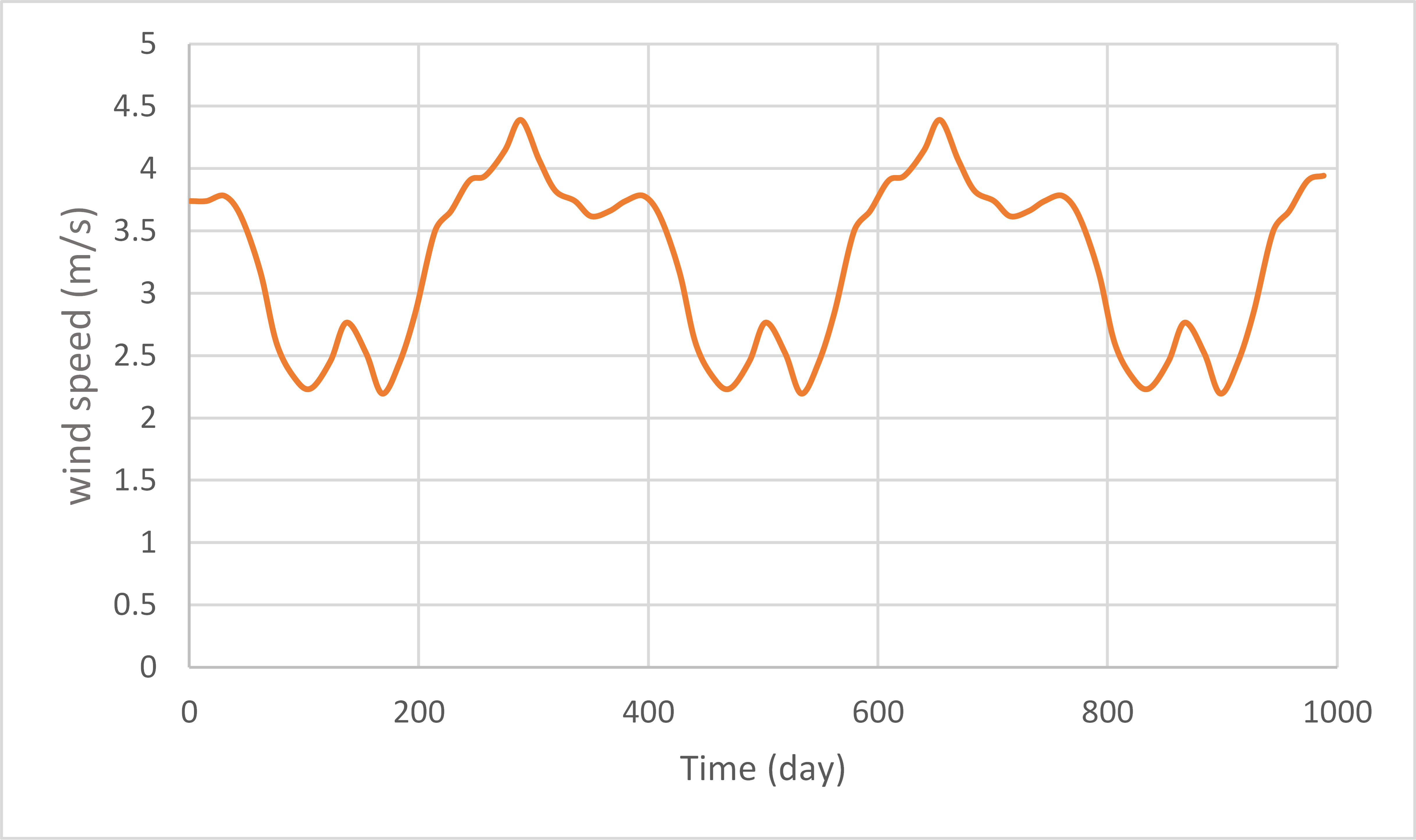
The data can be found in the tab “4. Air Temperature”, “5. Wind Speed”, “6. Evaporation”, “7. Solar Radiation”, “8. Albedo”, “9. Vegetation Height”, and “10. Snow Depth” respectively from the “Effects of thermosyphon on shallow foundation” Excel sheet. The graphs are also shown below.
Air temperature vs. Time
Wind speed vs. Time
Evaporation vs. Time
Solar radiation vs. Time
Albedo vs. Time
Snow depth vs. Time
- Required parameters are now defined. Select OK in the Define function dialog to apply Climate Flux as the time dependent function. The Set Boundary Conditions dialog should look as follows:
- To assign the condition in the modeler:
- Select Stage 2. Sept
- Select Group 1 segment
- Click Apply Condition in the Set Boundary Conditions dialog. The Climate Flux boundary condition will be added from Stage 2. Sept until the last stage.
- Select Group 2 segment in the modeler
- Click Apply Condition in the Set Boundary Conditions dialog
- Select Group 3 segment in the modeler
- Click Apply Condition in the Set Boundary Conditions dialog
The climate flux boundary condition has been applied to Groups 1 to 3 as separate items (Flux 3, Flux 4, and Flux 5 respectively under Visibility Tree) as follows:
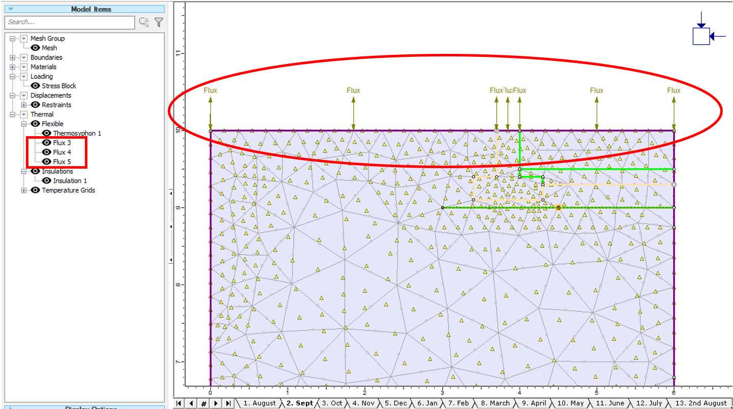
Note that the conditions are applied through Stage 2 to the last stage.
Let’s continue to define the boundary conditions for Groups 1 to 4 after building the structure.
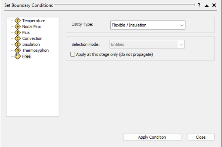
ii. Free Boundary Condition
- In the Set Boundary Conditions dialog, select Free from the left panel, Entity Type = Flexible /Insulation, as follows:
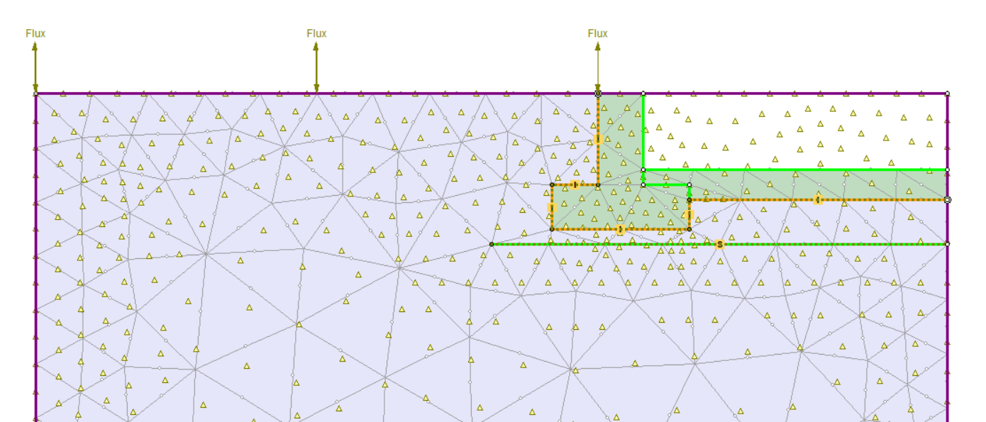
In the modeler: - Select Stage 13. 2nd August
- Select Group 2 and 3 segments
- Click Apply Condition in the Set Boundary Conditions dialog.
Now the top middle and right boundary segments (Group 2 and 3) are free from Stage 13 to the last stage.
iii. Temperature Boundary Condition
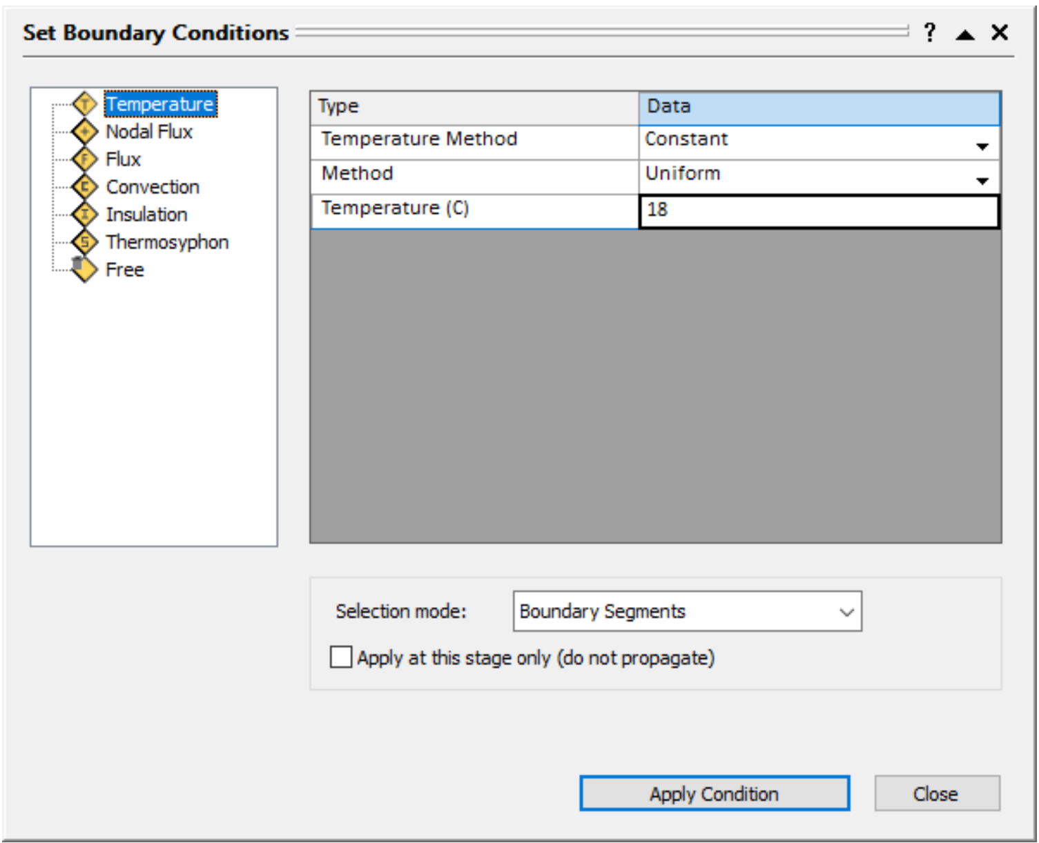
- In the Set Boundary Conditions dialog, select Temperature
from the left panel, set Temperature Method = Constant, Method = Uniform, and Temperature (C) = 18, as follows:
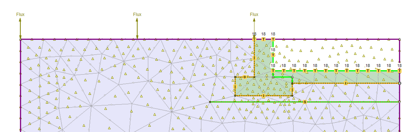
In the modeler: - Select Stage 13. 2nd August
- Select Group 2 and 4 segments
- Click Apply Condition in the Set Boundary Conditions dialog
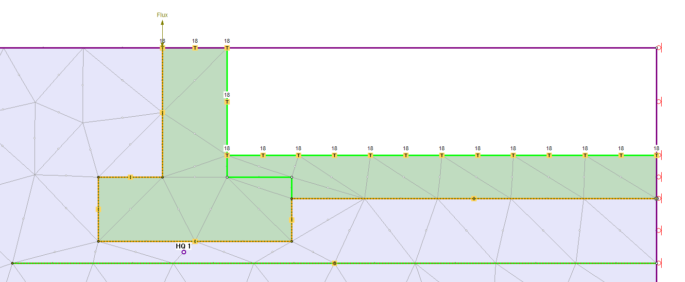
Now the top middle segment (Group 2) and the segments around the building (Group 4) have a constant temperature boundary condition of 18 C from Stage 13 to the last stage. The labels with a “T” letter and the temperature value “18” are marked along the boundaries, as follows:
Continue with Group 5 boundary conditions.
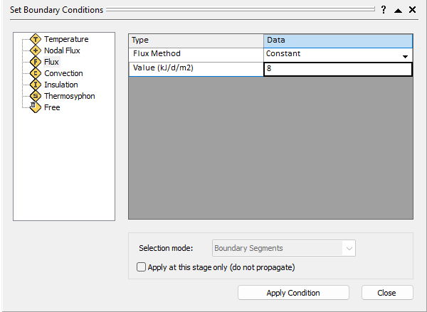
iv. Constant Flux Boundary Condition
- In the Set Boundary Conditions dialog, select Flux from the left panel. Set Flux Method = Constant, and Value (kJ/d/m2) = 8, as follows:
In the modeler: - Select Stage 2. Sept
- Select Group 5 segment
- Click Apply Condition in the Set Boundary Conditions dialog
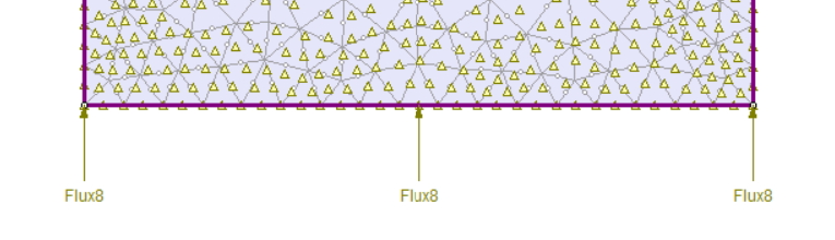
Now the constant flux boundary condition of 8 kJ/d/m2 has been added to the bottom boundary with the from Stage 2. Sept to the last stage. - Thermal boundary condition assignment for external boundaries is now completed. Click Close in the Set Boundary Conditions dialog.
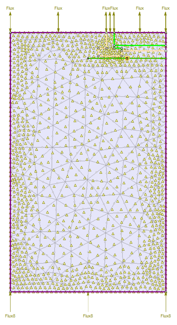
Before building the structure (Stage 2-12), the model domain has a climate flux boundary condition from the top, and a constant flux of 8 kJ/d/m2 boundary condition from the bottom. A thermosyphon is installed below the structure since stage 2. See the picture below.
After building the structure (Stage 13-24), an insulation boundary condition is applied along the joint boundary. The right part of the top boundary condition from the geometry has been changed to a constant temperature (18 C) boundary condition from the concrete structure. See the picture below.
| 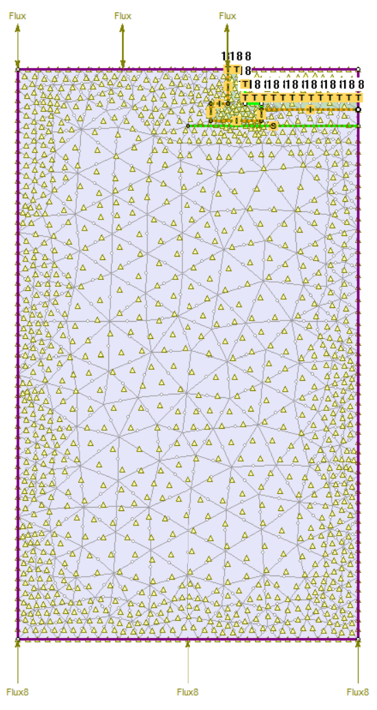 |
| a) Before building the structure | b) After building the structure |
2.8. Restraints

- Select: Restraints workflow tab
- Use Restraint X and Free options in Displacement menu. Free the top and internal restraints. Restrain X for side boundaries as follows:
2.9. History Query
- Select: Analysis > Add History Query

- Enter coordinate (3.8, 9.05), and press Enter. Press Enter again to exit. A history query point has been added between the concrete structure and thermosyphon, in order to investigate the historical data at that point.
The model construction is now complete. - Select: File > Save As
 to save the model as Effects of thermosyphon on shallow foundation (final).fez
3.0 Compute
- Select:
Analysis > Compute

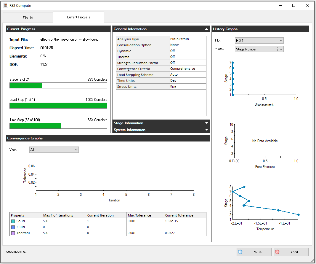
During compute, the progress data can be shown in Current Progress tab of RS2 Compute dialog. - Under the History Graph section, set Plot = HQ1
and Y-Axis = Stage Number to view the temperature change at History Query 1 through stages.
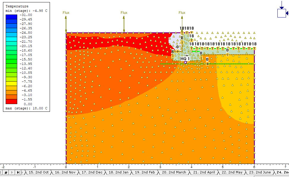
4.0 Results
- Select: Analysis > Interpret

- Select Thermal > Temperature
 from the drop-down menu. Right click on the screen, select Contour Options.
 - In the Contour Options dialog, choose Custom Range, set Min = -31 and Max = 0. Click Done to apply and exit the dialog.
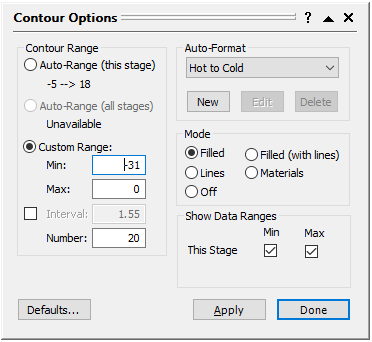
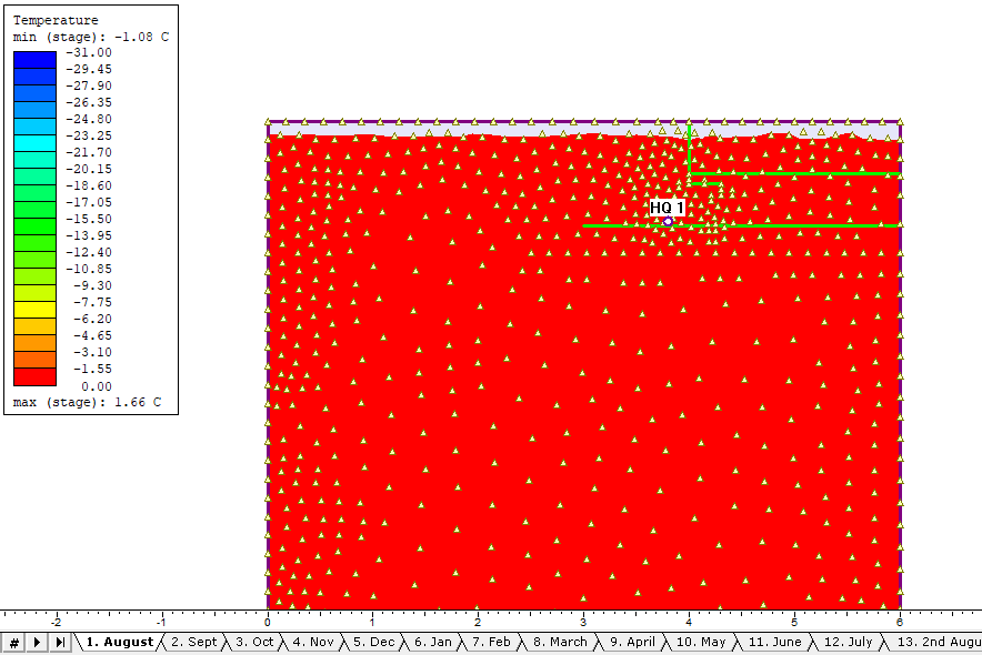
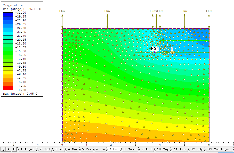
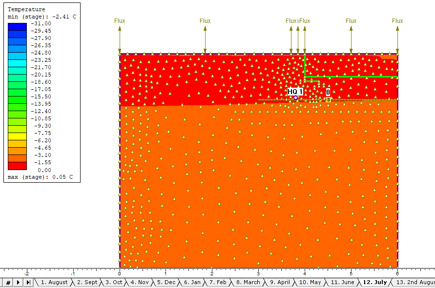
The temperature contours between -31°C and 0°C will be displayed.
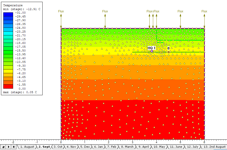
Compare temperature contour for stage 1 to stage 2, the temperature drops after thermosyphon installation, which demonstrates the thermosyphon has been activated.
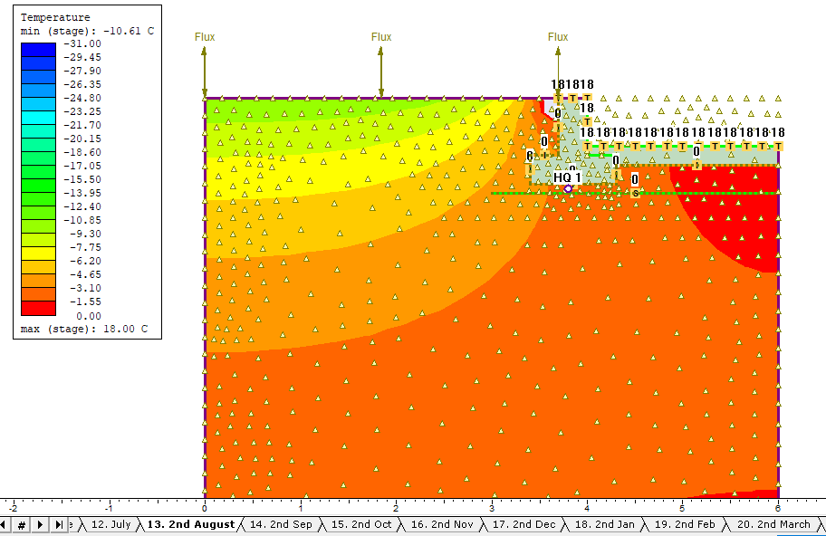
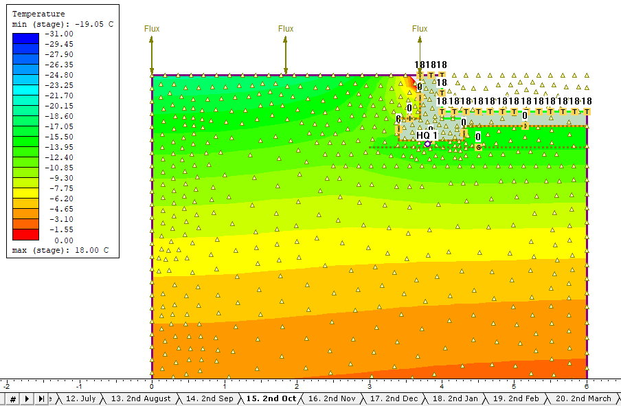
From stage 2 to stage 12, soil temperature at the region around the thermosyphon maintains below zero even in summertime. From stage 13 to 24, after building the structure, the soil temperature around the thermosyphon still stays below zero. Therefore, the installed thermosyphon is working effectively to keep the soil frozen.
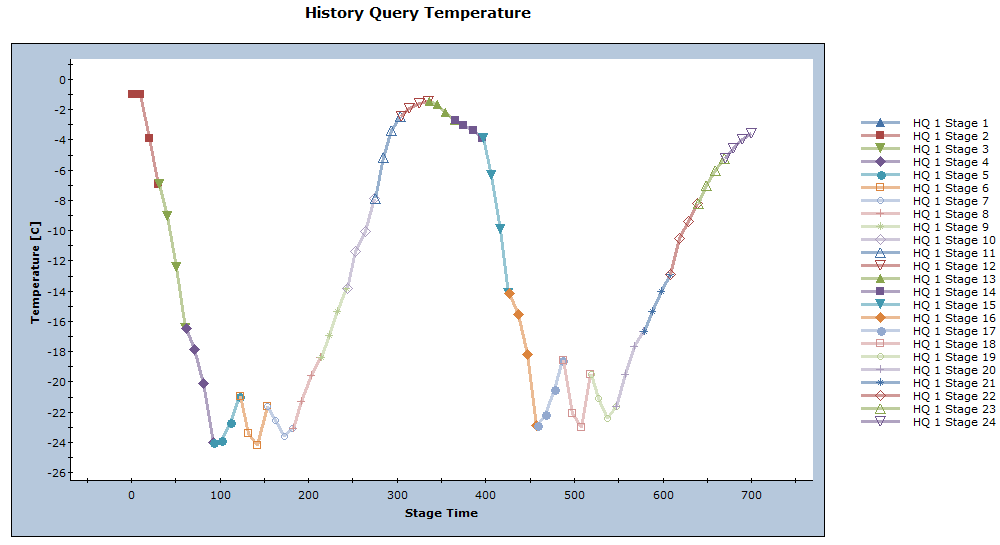
- Select: Graph > Graph History Query Data
 , select the HQ 1 point with the mouse, and press Enter (or right click on HQ 1 point and select Graph History Query Data).
 - In the Graph History Query Data dialog, select Vertical Axis = Temperature, Horizontal Axis = Time, select all stages, and press Plot. A graph indicating the temperature change throughout the analysis [Stage Time (days) vs. Temperature (C)] is plotted as shown below. It is evident from the plot that the soil underneath the structure stays frozen, permafrost has been maintained by using thermosyphon.
This concludes the tutorial.