Geogrid Reinforced Embankment

1.0 Introduction

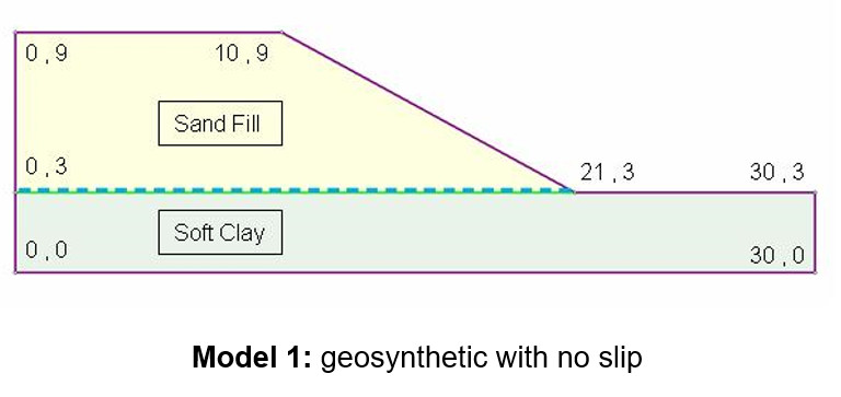
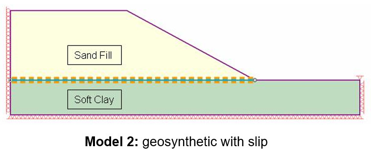
This tutorial demonstrates the use of geosynthetics in RS2 by performing a shear strength reduction (SSR) analysis for a sand embankment on top of a soft clay layer with a geogrid liner in between. The tutorial analyzes the results of two different models; in the first, the geogrid liner is fully bonded to both soil layers to prevent slip at the soil/geogrid interface, and in the second, the structural interface option is used to model support that has a sliding interface (joint) on both sides of the support element (i.e., simulating a geosynthetic with slip). The second model was constructed in two stages; the first stage simulates only the clay layer, while the geogrid and the sand fill embankment are added in the second stage. The model allows for slip between the geogrid liner and the soil layers. For additional information about adding structural interfaces, please visit the RS2 User Manual.

2.0 Compute (no slip)

1. Select: File > Recent Folders > Tutorial Folder
2. Open the starting file Geogrid Embankment file (no slip).
3. Select: Analysis > Compute

3.0 Results and Discussion (no slip)

1. Select: Analysis > Interpret

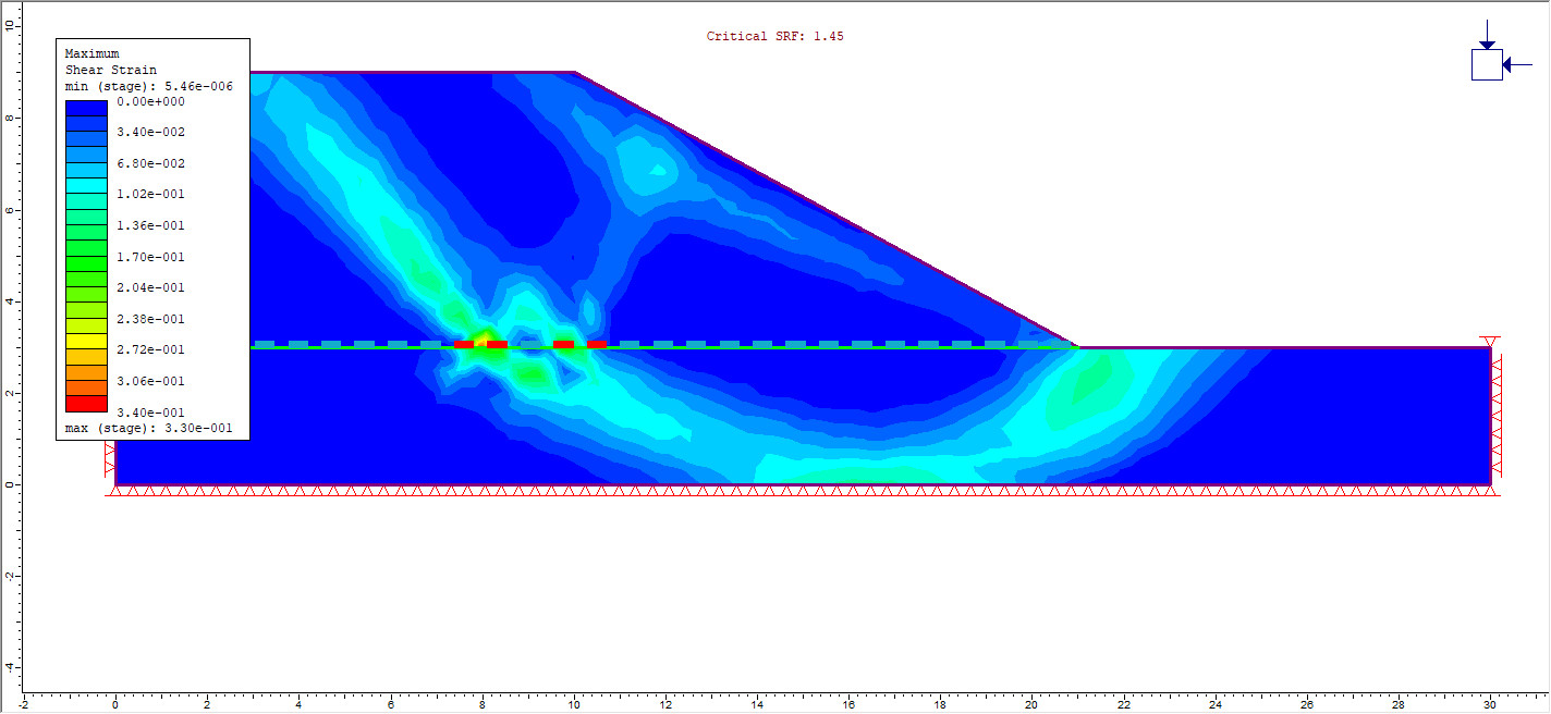
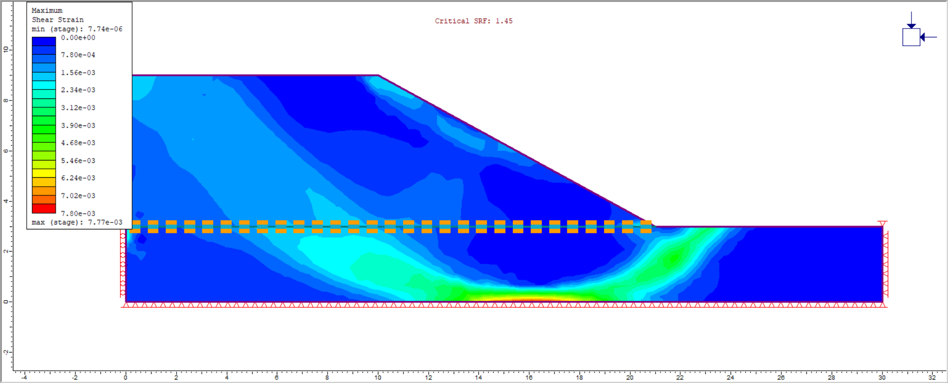
The following screen is displayed with the critical strength reduction factor (SRF written at the top of the window).

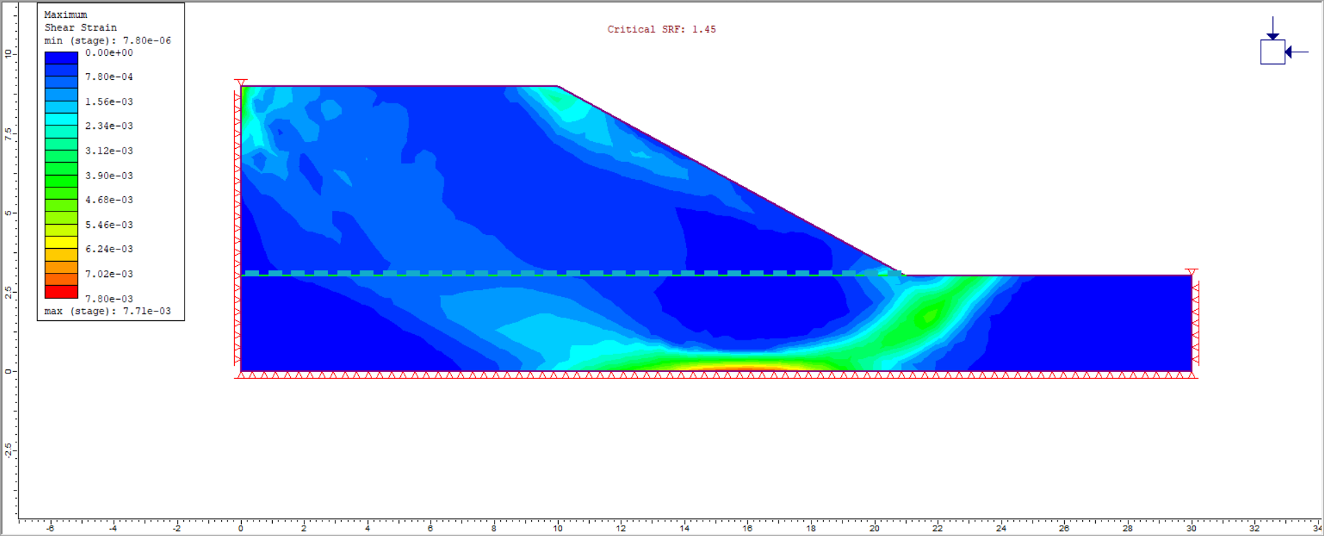
The Interpret view lists the various computed reduction factors in tabs along the bottom of the screen. The tab that is selected by default is the critical SRF. The maximum shear strain dataset is selected and contoured. Maximum shear strain gives a good indication of where slip is occurring, especially when viewing higher SRF values. Cycling through the various SRF tabs gives a good indication of the progression of failure through the slope.

1. Select: Display Yielded Liners in the toolbar.
2. There should be no change, indicating that none of the geogrid elements have failed.
3. Change the SRF to 1.46 by selecting the tab at the bottom of the window.

Observe that two of the geogrid elements have failed and that large shear strains accompany this failure.

The tensile failure of the geogrid has resulted in unstable sliding of the slope (lack of convergence in the model).

Switch to SRF: 1.75. Note the two well-formed shear bands in the model.

4.0 Constructing the Model (with slip)

1. Select: File > Recent Folders > Tutorial Folder
2. Open the file Geogrid Embankment file (without slip) - we will proceed by adding slip between the geogrid liner and soil layers and separating the model construction into two stages.

4.1 Project Settings

1. Select: Analysis > Project Settings
2. Select the Stages tab and enter Number of Stages = 2.
3. Click OK to close the dialog

Building the model with multiple stages and with slip is more realistic than the previous model analyzed in this tutorial that was constructed in one stage without slip. The first stage will consist of only the clay layer. In the second stage, we will then add the geogrid and the sand fill embankment. We do this by applying the following steps:

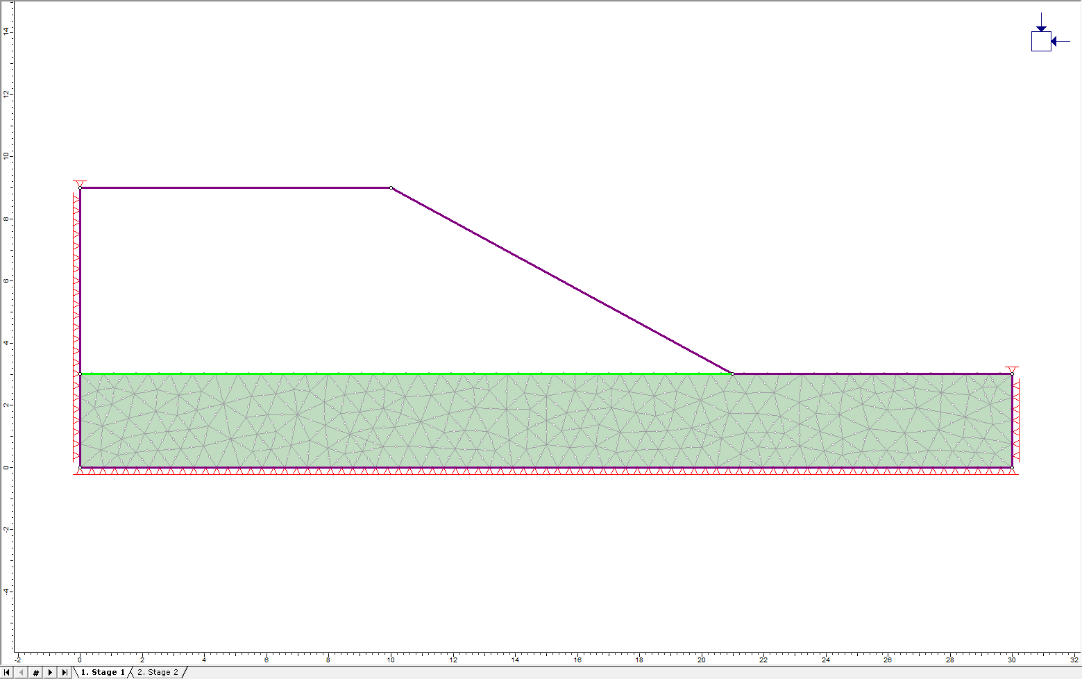
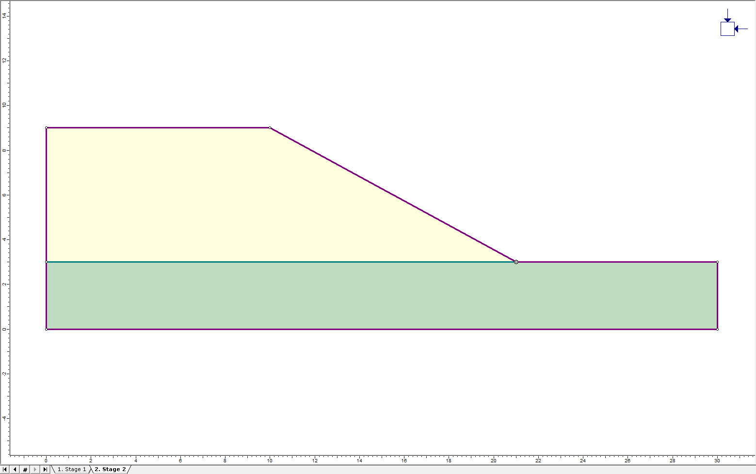
4. Click on the Stage 1 tab at the bottom of the window. Right-click inside the Sand Fill layer and choose Assign Material. A list of possible materials will now appear. Choose Excavate. This will delete the sand fill layer.
5. Right-click on the geogrid liner in the Visibility Tree and select "Delete from Model". The model should now appear as below:
   
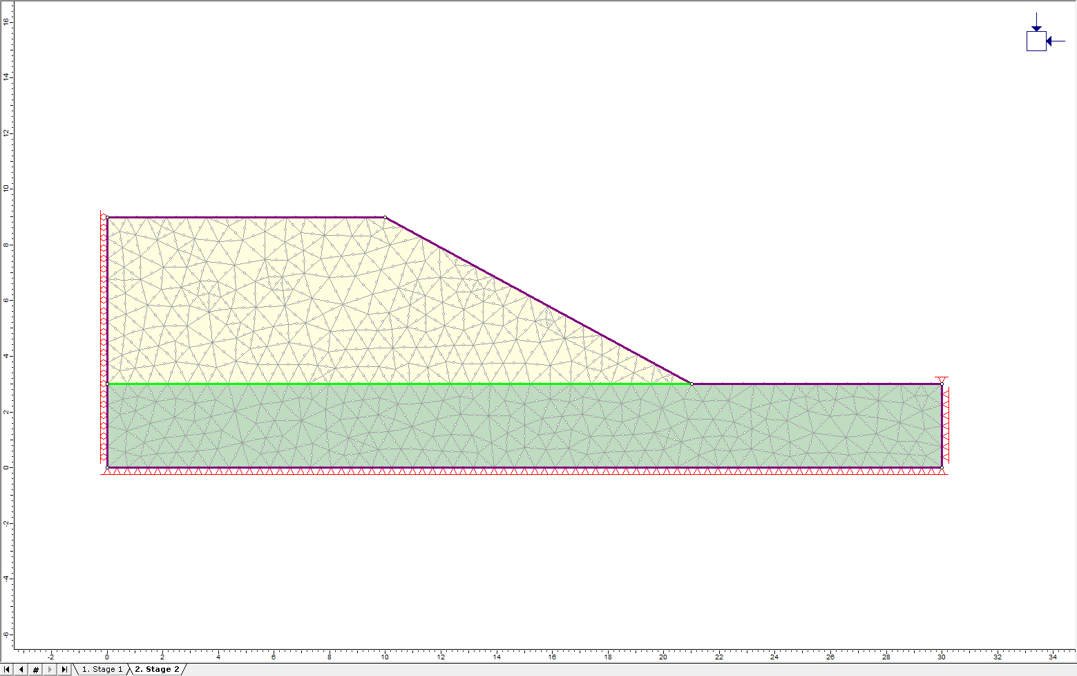
6. Click on the Stage 2 tab. Add the sand fill embankment by right-clicking in the excavated zone, choosing Assign Material, and then choosing Sand Fill.
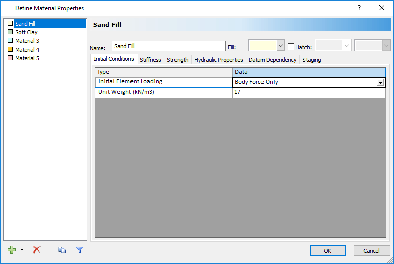
7. Since the sand fill is manually deposited on top of the existing clay layer, the sand fill will not have in-situ stress associated with it. The stress that develops in the sand fill will be purely due to its own weight. Therefore we need to change the sand fill properties. Right-click inside the sand fill. Select Material Properties. For Initial Element Loading select Body Force Only as shown. Click OK.
   
8. The sand fill will likely settle under its own weight. To enable this settlement, the left boundary must be allowed to move in the vertical direction. To do this, right-click on the left boundary of the sand embankment. Select Restrain X. The clay layer will also compact under the weight of the sand, so right-click on the left boundary of the clay layer and select Restrain X. Finally, the bottom left corner needs to be restrained both in X and Y, therefore right-click on the bottom boundary and select Restrain X,Y. The model should now look like this:
   

4.2 Geogrid Properties

To simulate a geosynthetic with slip, a Structural Interface should be used. The Structural Interface option in RS2 allows users to model support which has a sliding interface (joint) on BOTH sides of the support element. Therefore, both joint and liner properties must be assigned.

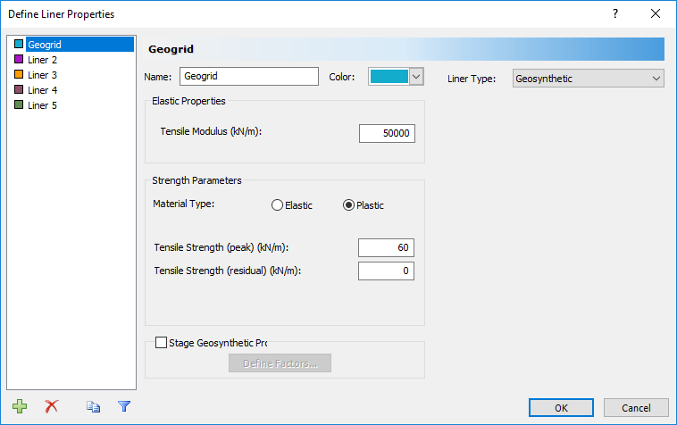
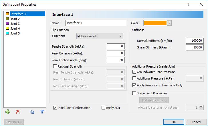
1. Select: Properties > Define Liners and Properties > Define Joints to set that the parameters are the same as below:
   
   
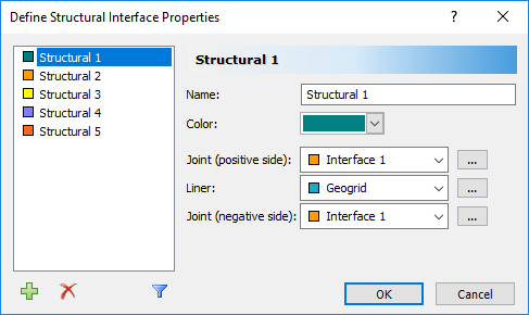
   Properties must be assigned to the Structural Interface.
2. Select: Properties > Define Structural Interface
3. The structural interface is composed of a liner sandwiched between two joints. Different combinations of liners and joints can be specified to make up a structural interface. Click OK in the window to use the existing values for joint and liner properties.
   

4.3 Adding the Structural Interface

1. Select: Boundaries > Add Structural Interface
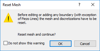
2. RS2 will prompt you to reset the mesh. Select OK in the warning dialog to reset the mesh:
   
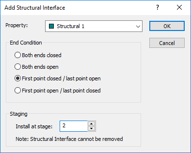
3. The "Add Structural Interface" dialog will appear. Choose "Structural 1" for the Property. Select "First point closed/last point open" for the End Condition.

If a joint end is closed, this means that the end of the joint boundary is represented by only ONE node in the finite element mesh, and therefore relative movement (sliding or opening) cannot occur at the joint end. If a joint end is open, this means that the end of the joint boundary is represented by TWO nodes in the finite element mesh, which can move with respect to each other. In this model, one end of the joint will terminate at a free surface (the toe of the embankment) so this end should be set to Open. The end of the structural interface within the embankment will be defined as closed. We only want the geogrid to be installed at Stage 2 of the simulation.

4. Set the Install at stage option to 2. The dialog should look like this:

TIP: After installing the structural interface, you can still alter the stage at which it is installed. To do this, view the desired stage and then right-click on the Structural Interface and select "Install At This Stage".

5. Click OK to close the dialog and begin the selection of the boundary points. Click on the two endpoints of the existing material boundary (coordinates 0, 3 and 21, 3). Be sure to click the left point first to ensure that this is the closed end of the Structural Interface. Right-click and choose Done or press Enter to finish. The Structural Interface will now appear as a green line with a circled triangle indicating the closed end and an open circle representing the open end as shown below:

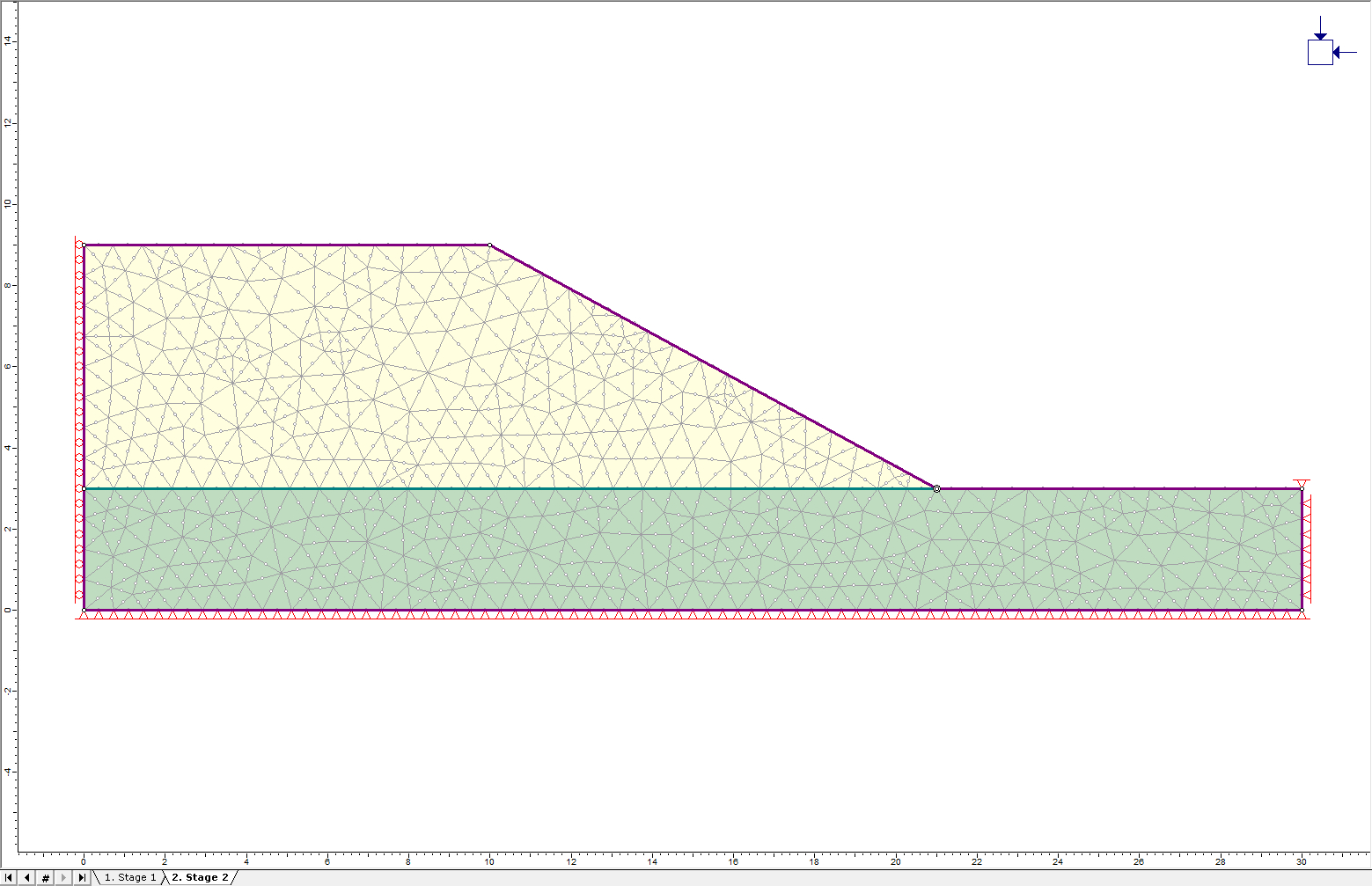
The geogrid has now been installed. The model must be re-meshed before computation.

6. Select: Mesh > Discretize and Mesh
7. Model construction is now complete. Save the model as Geogrid (with slip), then proceed with computation. The final model should appear as below:

8. Select: Analysis > Compute

5.0 Results and Discussion (with slip)

1. Select: Analysis > Interpret

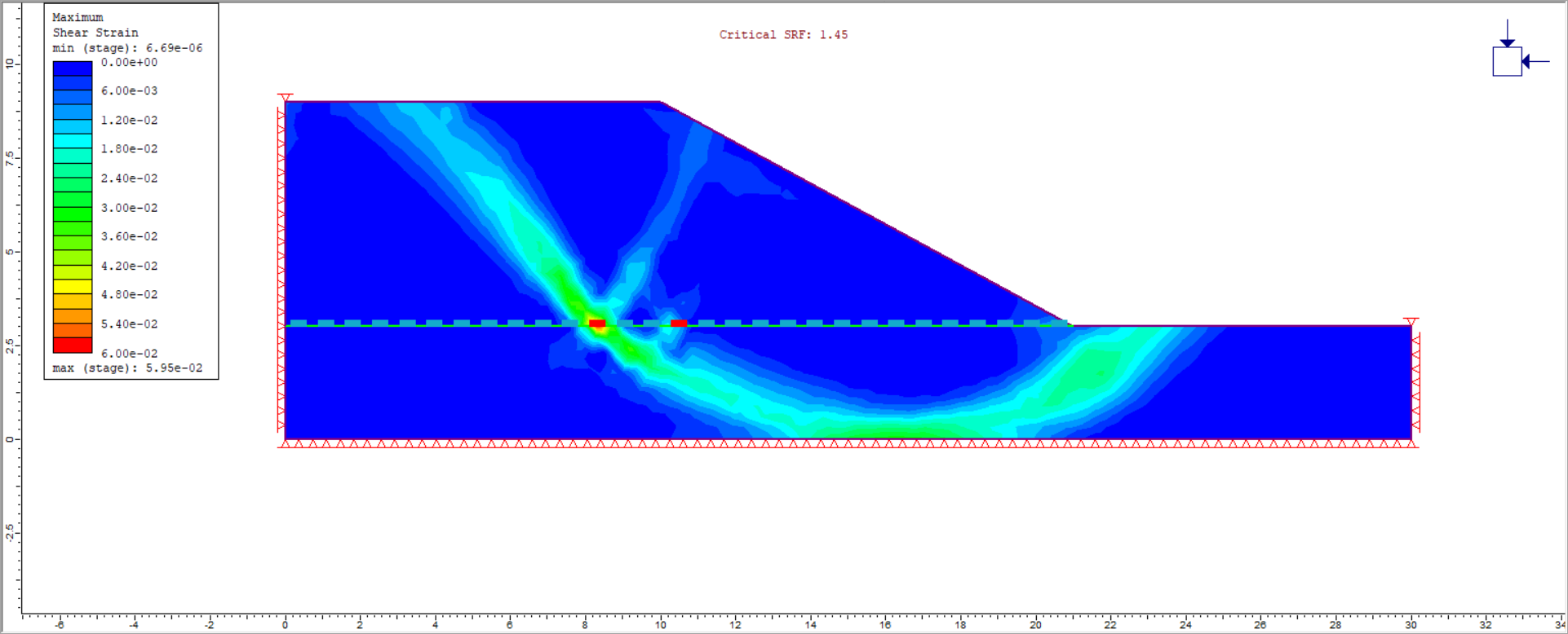
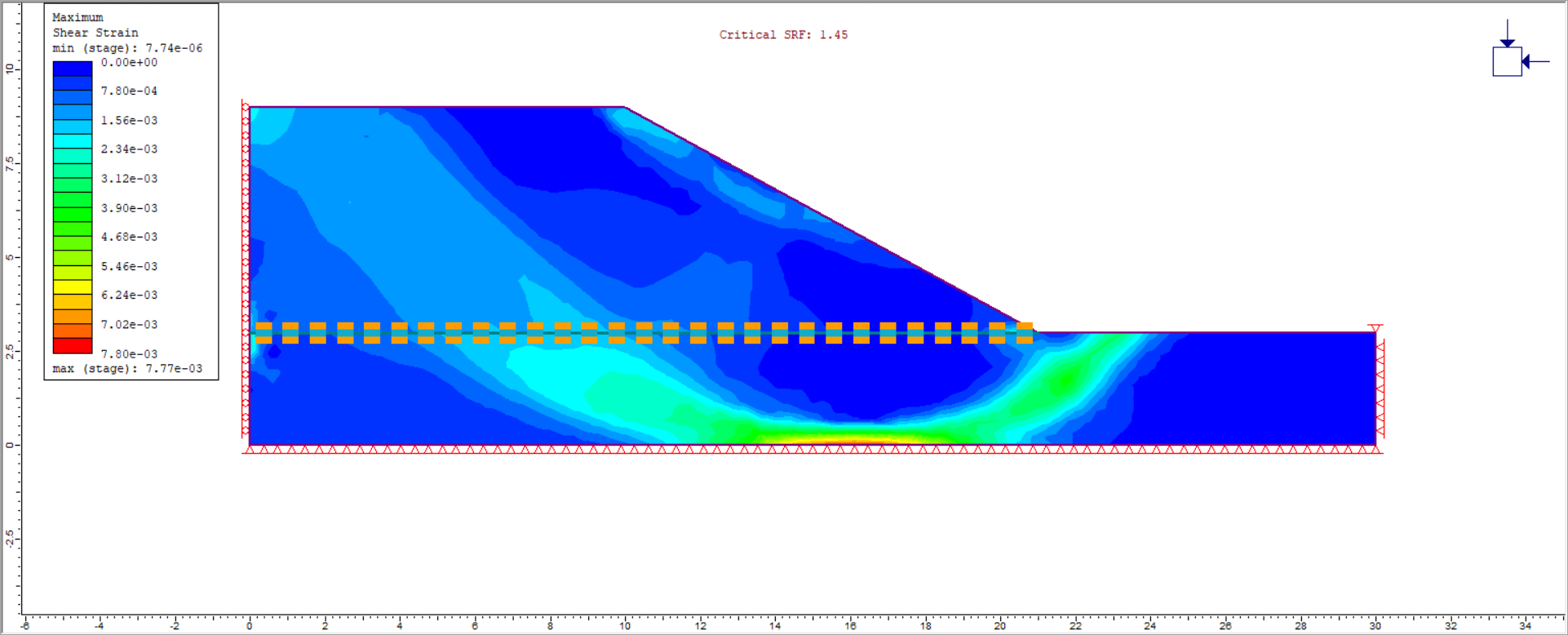
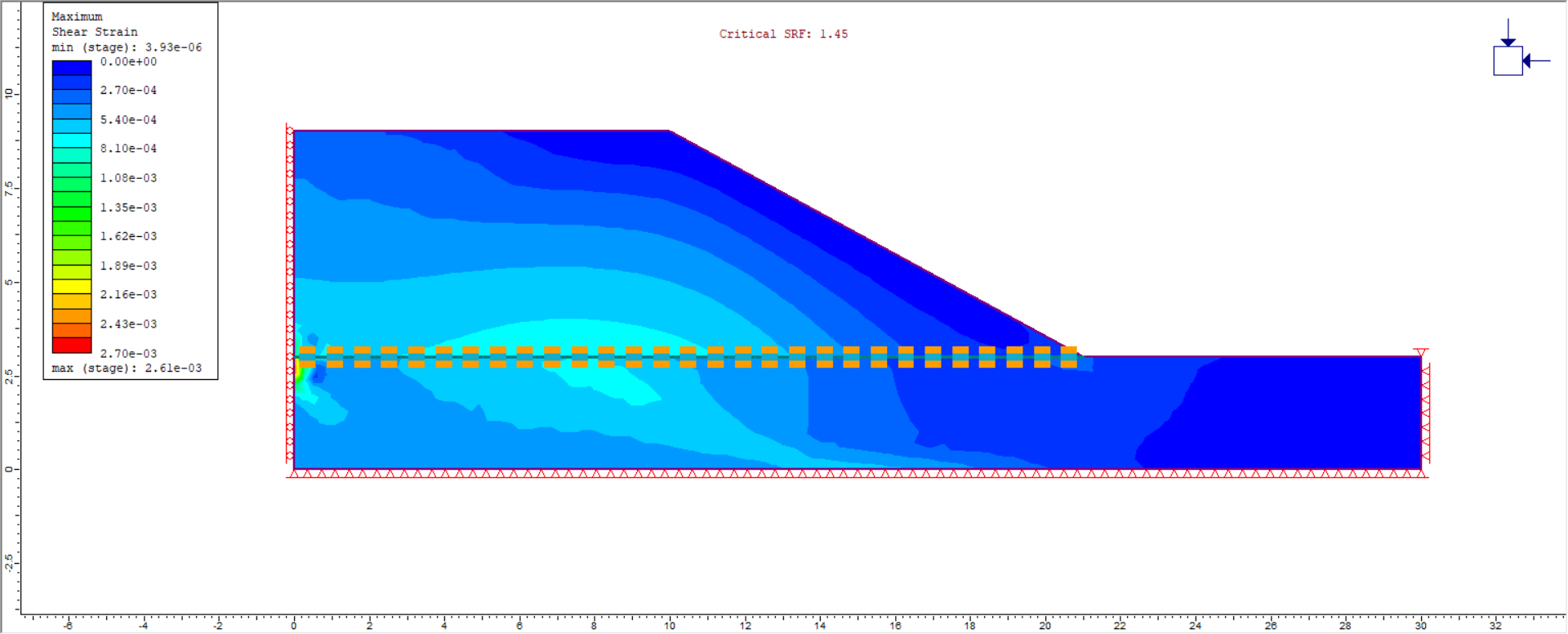
The following screen shows the Maximum Shear Strain contours at the critical Strength Reduction Factor:

Before looking at the Shear Strength Reduction analysis, let’s check the effect of the staging. The stress analysis results of Stage 1 and Stage 2 are not available to view; only the data for the different SRF values are available. To view the results from the different stages:

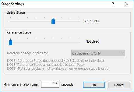
2. Select: Data > Stage Settings
3. Move the reference stage slider all the way to the left so that it reads “Not Used”.
4. Click OK button to exit the dialog.
   

Stage 1 and Stage 2 tabs now exist along with the SRF tabs at the bottom of the view.

5. Select the Stage 1 tab to view Stage 1 results.
6. After selecting the Stage 1 tab, plot contours of maximum stress by choosing Sigma 1 from the drop-down menu on the toolbar.
   

The model should appear as follows:

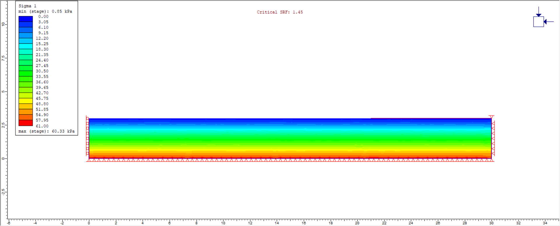
As expected, the stress increases with depth in the clay layer due to gravitational load. This stress is mostly due to the initial element loading. Plotting displacements will show that almost no displacement has occurred.

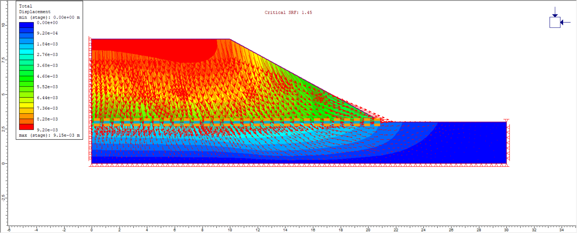
7. Click on the Stage 2 tab. Larger stresses under the sand embankment are visible.
8. Change the contours to plot displacements by choosing Total Displacements from the drop-down menu on the toolbar.
9. Show the deformation vectors by selecting the Display Deformation Vectors button.

A large amount of vertical displacement occurred in the sand and the clay as the soil layers compacted under the weight of the sand.

10. Click on the SRF=1 tab.

The results will appear the same. This is because SRF: 1 means that no strength reduction has been applied, so these results are the same as the Stage 2 results.

To look at deformations caused by strength reduction, rather than by settlement, go back to the Stage Settings item in the Data menu and set the reference stage back to SRF 1.

11. Now go back to the plot of SRF: 1.45 and change the contours back to Maximum Shear Strain.
12. Turn off the displacement vectors.
13. Display the yielded elements in the geogrid.

It is apparent that joint elements at the toe of the embankment have failed (slipped). Slippage has occurred on both sides of the geogrid, i.e. between the liner and the sand, as well as between the liner and the clay.

14. Go back to the plot for SRF: 1.

The same slippage has occurred, even before any shear strength reduction. This shows that the weight of the sand material has caused slip along the geogrid material interfaces, but that this slip is not responsible for the failure of the slope.

15. Now change the SRF to 1.45 by clicking on the SRF: 1.45 tab at the bottom of the window.

Observe that elements in the geogrid itself have failed and that large shear strains accompany this failure.

The tensile failure of the geogrid has resulted in unstable sliding of the slope (lack of convergence in the model).

16. Click through the other SRF plots to see further failure in the geogrid and the evolution of two localized shear bands.

5.1 GRAPHING GEOGRID DATA

A graph of the tensile force acting on the geogrid can be easily obtained.

1. Select: Graph > Graph Liner Data
2. Click on the geogrid line and press Enter.
3. A dialog will appear asking which data to plot. Use the defaults for the Vertical Axis and Horizontal Axis. Under Stages to Plot, turn on SRF: 1.45 and SRF: 1.46. Turn off the other ‘stages’. Recall that the different SRF models are considered as different stages in RS2.
You can perform the same task by right-clicking on the geogrid liner and choosing Graph Liner Data.
4. Select Plot.

This will generate a graph of axial force along the length of the geogrid liner for the two SRF models.

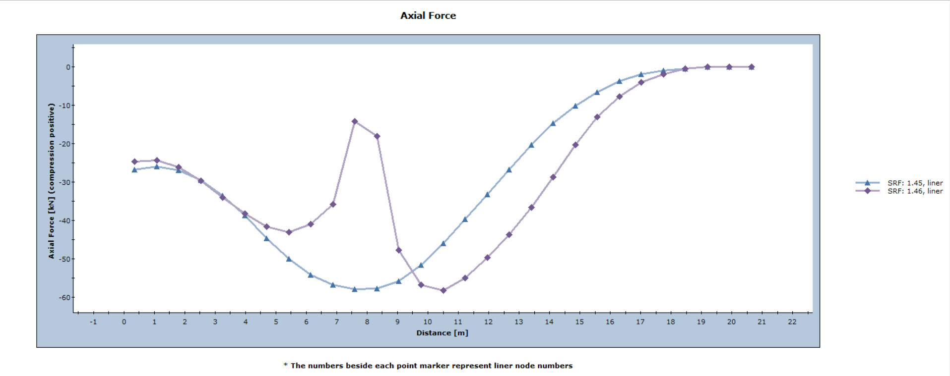
This graph shows the tensile (negative) forces supported by the geogrid. Recall that the geogrid cannot support compressive forces. The failure of two elements in the SRF: 1.45 model has caused a drastic drop in the tensile forces compared with the SRF 1.46 model. This loss of support in the geogrid is what leads to the slope failure in the model.

Try re-running the model with no geogrid liner. Observe that the critical SRF is 1.26 and that the failure surface is less localized.

This concludes the Geogrid Embankment Tutorial.