Dynamic Slope Analysis A

Deconvolution of the Earthquake Input

1.0 Introduction

Design earthquake ground motions are usually provided as outcrop motions. However, for an RS2 earthquake analysis, seismic input must be applied at the base of the model rather than the ground surface. Therefore, it is necessary to “deconvolute” the given data, so once it is applied at the base of the model, it correctly simulates the design motion.

Given the acceleration-time history, this tutorial will take steps to demonstrate that the dynamic load applied to the top of the model simulates the same motion as it applied to the base:

1. Integrate the given acceleration-time history to obtain velocity with baseline correction.
2. Apply the velocity to the top of the model.
3. Apply the velocity to the base of the model, using the “Compliant base” option. This option converts the inputted velocity data to stress.

This input stress defines the upward wave motion into the model. However, the actual motion at the base is the superposition of the upward and downward wave motion reflected from the model.

The top of the model is a free surface – there is zero shear stress at the free surface. Therefore, for this to be true, the upward and downward waves at the top of the model must be equal, and the velocity history applied at the base of the model must be equal to the given outcrop motion.

2.0 Constructing the Model

1. Select File > Recent Folders > Tutorial Folder
2. Open the Dynamic Slope Analysis Part A (Initial).fez file.

The model already has project settings defined (tick box for Dynamic Analysis in Project Settings), an external boundary created, and material properties defined. The nodes on the sides of the column have been tied together by an element edge without any internal nodes and given a tied boundary condition setting; therefore, the mesh was set up using the “no internal nodes” type and elements without midside nodes.

2.1 Restraints

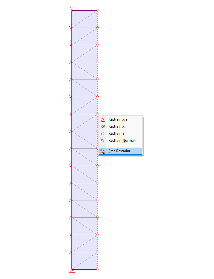
The soil column has been restrained by default. The lateral sides of the model need to move freely.

1. Right-click on each of the lateral boundaries of the column and select: Free Restraint.

Let’s place a restraint at the bottom of the column; this will be removed in Stage 2.

2. Select: Displacements > Set Displacement
3. Enter Displacement in X direction = Displacement in Y direction = 1.
4. Check the “Stage displacements” box and click on the Stage Factors button.
5. In the dialog, change the factor of Stage 1 to zero. Check the Free box for Stage 2.

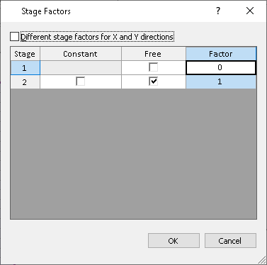
A factor of zero represents a zero-displacement boundary condition. The free check box means that the nodes in Stage 2 are free to move without restraint. A factor of 1 means that the displacement will be equal to the magnitude(s) entered in the Nodal Displacement dialog.

Therefore, all restraints have been removed in Stage 2, and a zero-displacement boundary condition set in Stage 1.

6. Select OK in the Stage Factors dialog and select OK in the Nodal Displacement dialog.
7. Using the resulting selection tool, click on the bottom boundary and press Enter.

The model should look as follows in Stage 1:

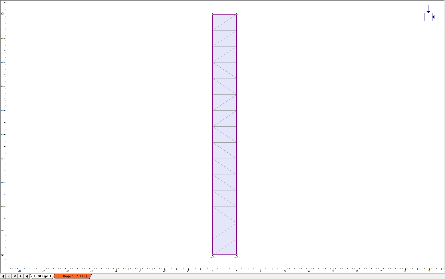
Now click on the Stage 2 tab at the bottom left of the window. Notice that Stage 2 has no restraints, as expected.

2.2 Time Query

Several time steps will occur between the defined stage times; RS2 will not output data for all the nodes for these intermediate time steps. However, the modeler allows the user to specify time query points in the mesh. Time Queries record the dynamic data for all dynamic time steps occurring in the simulation. For this model, one time query will be created.

1. Select: Dynamic > Time Query > Add Solid Time History Query
2. Clicking on a point will place a query at that point, or the exact coordinates may be typed in. Add a time query point at the following location on the column: (1, 10). Press Enter after selecting the coordinate.

2.3 Boundary Conditions

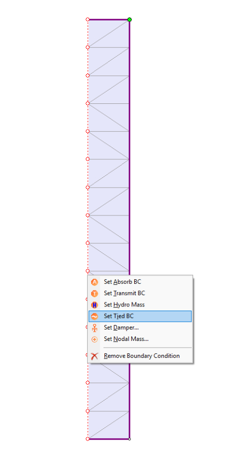
1. Ensure the Dynamic workflow tab is selected for Stage 2 of the model. Right-click on one of the lateral sides of the column and select “Set Tied BC,” as shown. Do this for both lateral sides of the column.
   
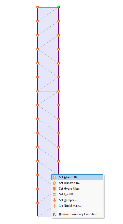
2. Then, right-click on the bottom boundary and select “Set Absorb BC.”
   
   
3. The base model is now complete. Save the model from the File menu as “Model 2.” Then select File > Save As and save another copy as Model 1.
   

3.0 Results and Discussion: Model 1

In Model 1, the original acceleration-time history data for the 1985 Mexico City earthquake need to be adjusted with baseline correction in the order to measure site data error. Using RS2 Dynamic Data Analysis function, the adjusted velocity data can be obtained, and will be inputted to the top of the model.

The original acceleration-time history data can be found in the Excel Sheet in the installation folder. For Windows 7 and 8 the file path is:

C:\Users\Public\Documents\Rocscience\RS2 2019\Examples\Tutorials

1. Open the Excel file titled “Mexico City 1985 - Mesa Bivradora C. U.”
2. Ensure the first sheet, titled “Mexico City 1985” is selected.
3. In RS2, select the Dynamic workflow tab.
4. Select Dynamic > Dynamic Data Analysis

We will now copy and paste the data from the Excel sheet into the Dynamic Data Analysis dialog.

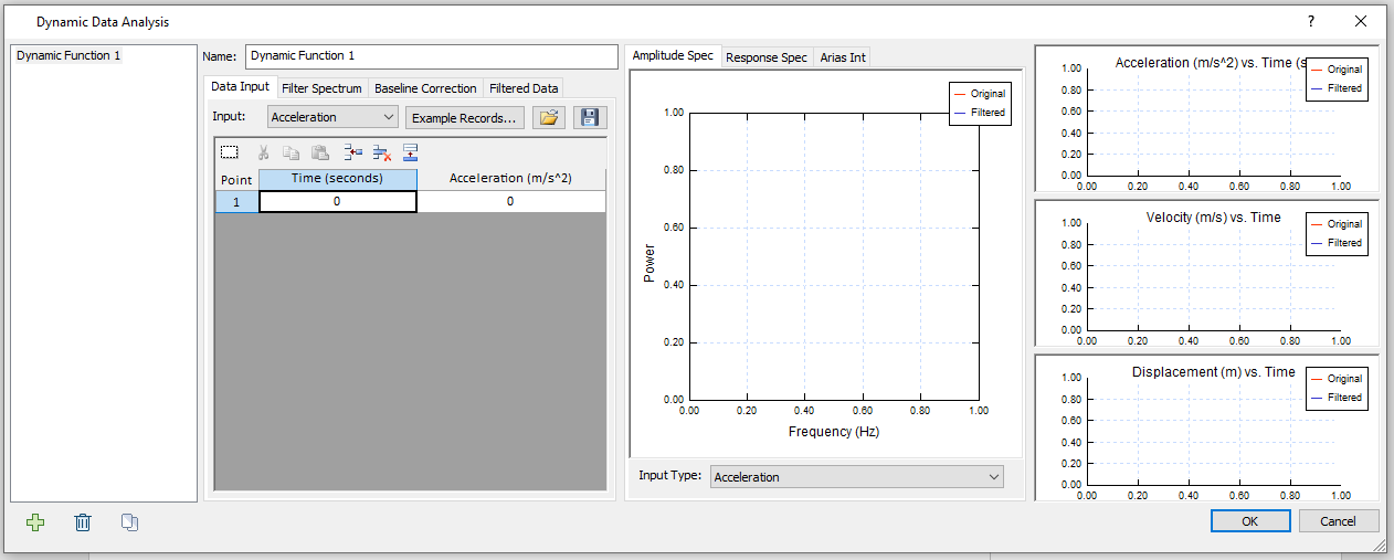
5. In the Dynamic Data Analysis dialog, ensure Data Input tab is selected, and Input = Acceleration.
6. Click on cell A6 in the first sheet of the Excel document. Then use the following shortcut to select the cells: CTRL + SHIFT + ↓
7. All cells from A6 to A3006 should have been selected, i.e. the time data. Copy this data (CTRL + C).
8. Returning to the Dynamic Data Analysis dialog in RS2, click on the name of the Time column to select the column, as shown:
9. Now, paste the time data into the column by clicking the paste button in the dialog or using the CTRL + V shortcut.
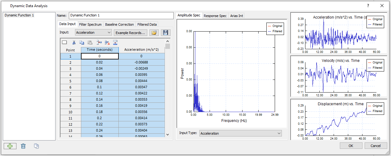
10. Follow a similar procedure to copy and paste the acceleration data (B6 to B3006) in the Acceleration column.

In the middle section of the dialog, make sure Input Type = Acceleration to show the Power vs. Frequency (Hz) plot based on acceleration data.



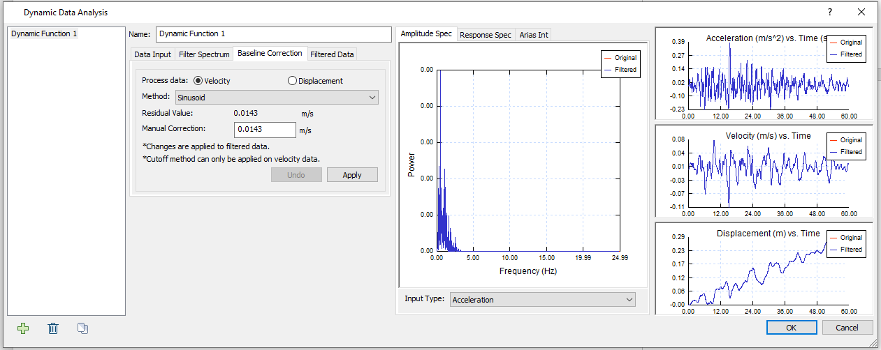
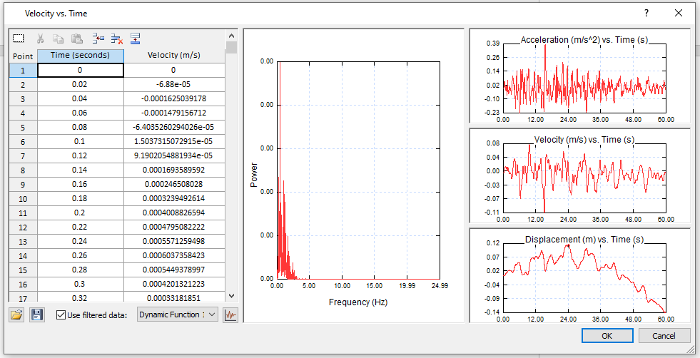
11. Select the Baseline Correction tab, ensure Process data = Velocity and Method = Sinusoid. The current residual value is given as 0.0143 m/s. Your dialog should look as the following:
12. Click Apply to apply Manual Correction of 0.0143 m/s. Now your dialog should look like the following:

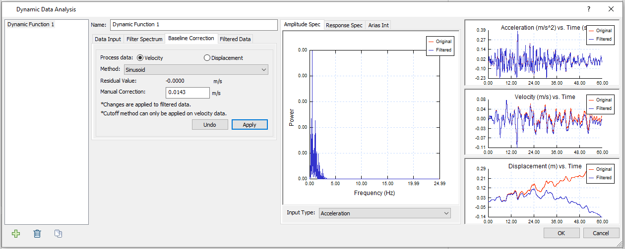
Now the residual value has been changed to 0 m/s, meaning the baseline has been corrected to 0 m/s. In Acceleration (m/s^2) vs. Time (s) and Velocity (m/s) vs. Time plots, amplitude loss exists but not significant, while the change is remarkable in the Displacement (m) vs. Time plot.

Here, the baseline correction is to make adjustment to measure site data error.

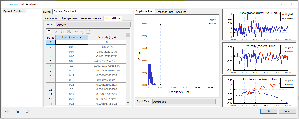
13. Select the Filtered Data tab as the following.

The filtered data are displayed, and the data type can be selected with the Output dropdown bar.

We will apply velocity output data to top of the model.



14. Click OK to close the Dynamic Data Analysis dialog.
15. Select Dynamic > Define Dynamic Loads
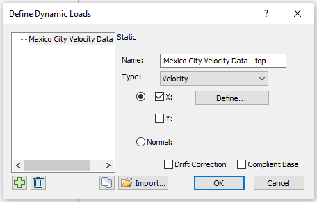
16. Rename “Dynamic Load 1” to “Mexico City Velocity Data - top.” Change the Type to Acceleration. Make sure both “Drift Correction” and “Compliant Base” options are unchecked. The dialog should look as follows:
    
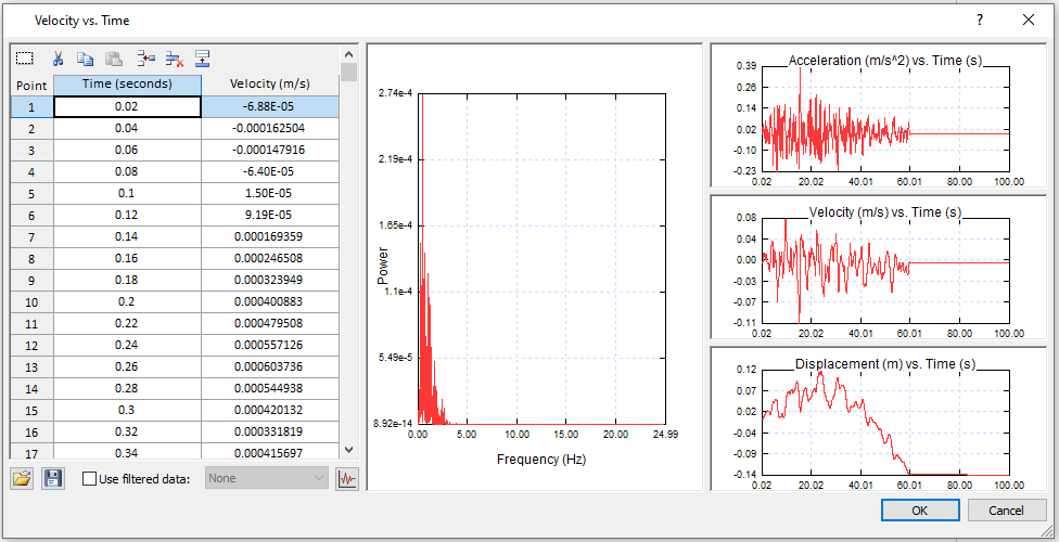
17. Now click the Define button beside X. In the Velocity vs. Time dialog.
18. Select the Use filtered data option at the bottom of the dialog and select Dynamic Function 1. Velocity output data from Dynamic Function 1 will be applied.

Your dialog should look as follows:



19. Click OK in both the Velocity vs. Time dialog and the Define Dynamic Loads dialog.
20. Select: Dynamic > Add Dynamic Load
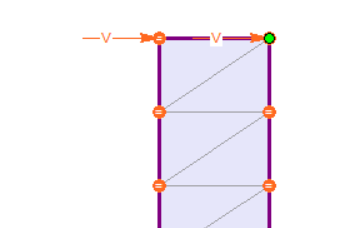
21. In the Add Dynamic Load dialog, the Load Function should be the dynamic load we have just defined, installed at stage 2. Click OK. Using the selection tool, click on the top boundary and press Enter.

The boundary should look as follows:

Let’s view the results.

1. Select: Analysis > Compute
2. Select: Analysis > Interpret
3. Click on the Stage 2 tab at the bottom left of the window to view the results.
4. Right-click on the time query point at the top of the model and select “Graph Time Query Data.” Set the Vertical Axis to “X velocity,” the Horizontal Axis to “Time,” and click Plot. The graph should appear as follows.
   
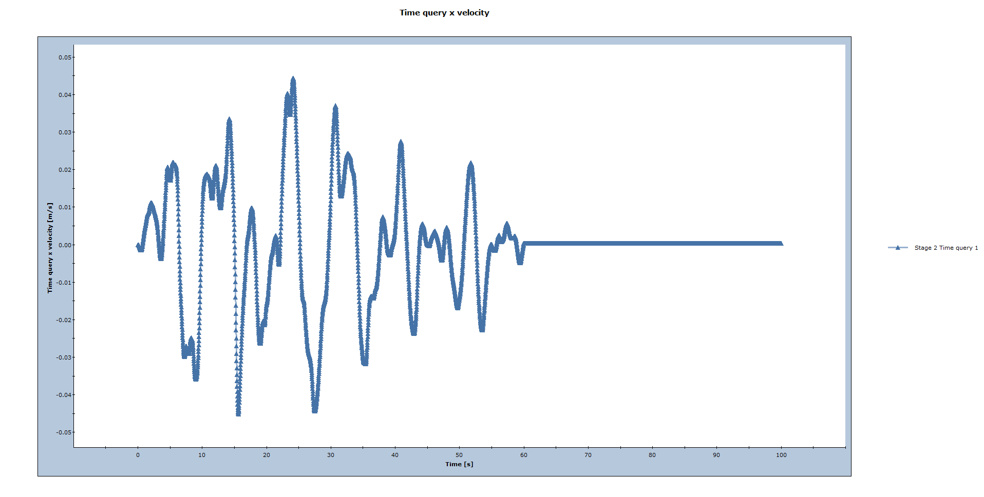
5. Right-click on the plot and select “Plot in Excel.” View the second sheet, containing the numerical data.
   

In the Spreadsheet, the velocity data, “Time query x velocity [m/s],” will be used in Model 2 later. (NOTE: These values can be found in Sheet 2, Column A and B of the Mexico City Excel file.)

6. Close Interpret and save Model 1.

4.0 Results and Discussion: Model 2

In Model 2, the Model 1 velocity results will be applied to the base of the model. We will set up from Model 1. Now let’s go back to Model 1 in RS2.

Ensure that the Dynamic workflow tab in Stage 2 is selected.

1. Select: Dynamic > Define Dynamic Loads
2. Click on the “Add a new dynamic load definition” button at the bottom left of the Define Dynamic Loads dialog. Rename “Dynamic Load 2” to “Mexico City Velocity Data - bottom.” Change the Type to Velocity, keep the “Drift Correction” option unchecked, and select the “Compliant Base” checkbox.
   
   The dialog should look as follows: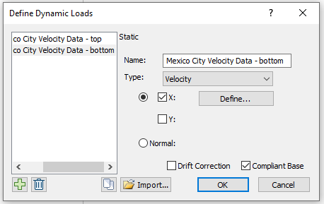
   
3. Now click the Define button and copy and paste the time data and the computed velocity data from the Model 1 (NOTE: These values can be found in Sheet 2, Column A and B of the Mexico City Excel file.). The dialog should look as follows:
   
   
4. Click OK in the dialog and click OK in the Define Dynamic Loads dialog.
5. Select: Dynamic > Delete Dynamic Load
6. Use the selection tool, click on the top boundary and press enter to delete the velocity load.
7. Select: Dynamic > Add Dynamic Load
8. In the resulting dialog, the Load Function should be “Mexico City Velocity Data – bottom (Velocity)” and it should be installed at stage 2 as follows:
   
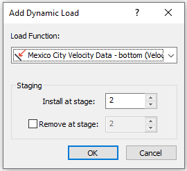
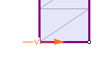
9. Click OK. Using the selection tool, click on the bottom boundary and press Enter. The boundary should look as follows:
   

Let’s view the results.

1. Select: Analysis > Compute
2. Select: Analysis > Interpret
3. Click on the Stage 2 tab at the bottom left of the window to view the results.
4. Right-click on the time query point at the top of the model
• Select: Graph Time Query Data.
• Set the Vertical Axis to “X velocity” and the Horizontal Axis to “Time,” and click Plot.
• Right-click on the plot and select “Plot in Excel.”
• View the second sheet, containing the numerical data.

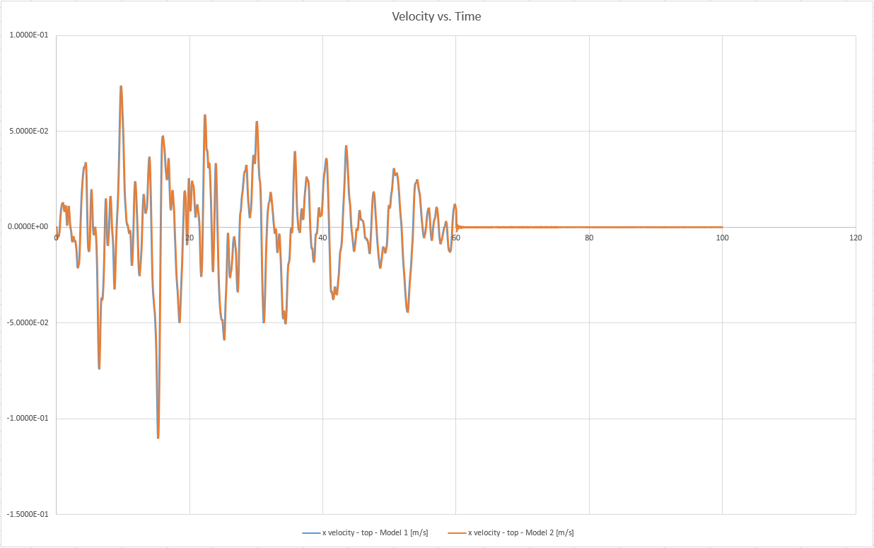
Let’s plot the bottom velocity values from this plot (Sheet 3, Column B) and the top velocity values from Model 1 (Sheet 2, Column B) on the same plot in Excel.

The plot (which can be found in Sheet 4 of the Excel file) should look as follows:

As expected, the two velocities are almost identical. Therefore, the velocity history applied at the base of the model is equal to the given outcrop motion.

This concludes the Dynamic Slope Analysis Part A Tutorial.