Dynamic Slope Analysis D

Dynamic Slope Stability

1.0 Introduction

This tutorial will outline a recommended procedure to simulate a seismic loading of a slope with RS2, followed by an analysis of the results.

The modelling procedure includes 5 steps:

• Deconvolute the given acceleration earthquake data (using drift correcting, filtering, etc.) (See Tutorial A and Tutorial B).
• Calculate the equilibrium state.
• Apply dynamic conditions.
• Determine damping Rayleigh of the model (See Tutorial C).
• Run the model with determined damping Rayleigh parameters.

This tutorial will start with the undamped model from Tutorial C; see this tutorial for a more in-depth explanation of how this file was created.

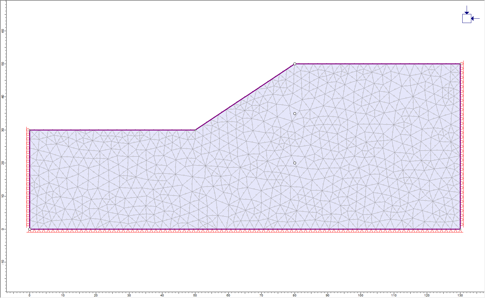
2.0 Constructing the Model

This tutorial uses the earthquake data from the 1985 Mexico City earthquake. The earthquake data has been deconvoluted (see Tutorial A) as well as filtered (see Tutorial B). We will use the undamped model we created in Tutorial C.

1. Open the Dynamic Slope Analysis C (Undamped Model).fez file from the Tutorials folder.

2.1 Project Settings

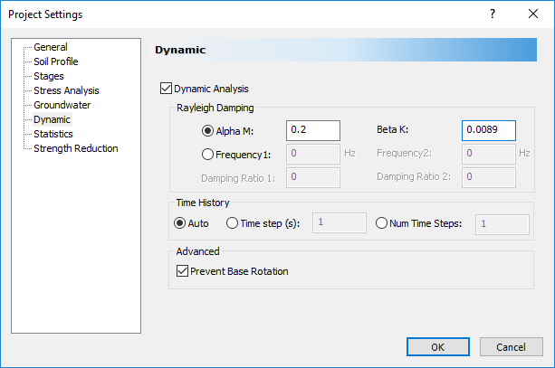
1. Select: Analysis > Project Settings
2. Select the Dynamic tab. In Tutorial C, the Rayleigh damping coefficients were determined to be αM = 0.2 and βK = 0.0089. Enter these values in the dialog:

We will also add three more stages to the analysis, to get a better idea of the results.

3. Click on the Stages tab in the Project Settings dialog and add one more stage to the analysis. Define the following names and ending times for each stage:

#	Name	Time (seconds)
1	Stage 1	0
2	Intermediate 1	5
3	Intermediate 2	10
4	Intermediate 3	45
5	Final Stage	100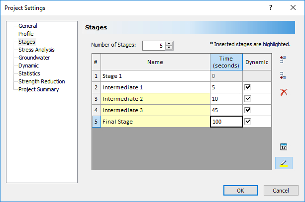



4. Click OK to close the Project Settings dialog.

This model uses a Plastic Material, instead of the Elastic one we used in Tutorial C.

5. Select: Properties > Define Materials
6. Select the Strength tab. For Material 1, change the Material Type to Plastic. Let’s use a Residual Tensile Strength of 5 kPa, a residual friction angle of 38 degrees, and a residual cohesion of 5 kPa, as shown.
   
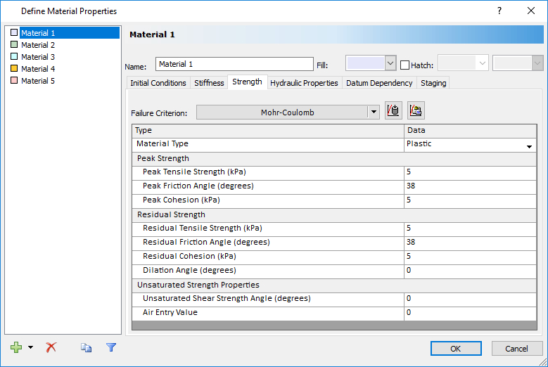
7. All other values will remain the same. Select OK to save the changes to the material properties.
   

2.2 Dynamic Loading

Let’s filter the dynamic load data we have applied to the model, based on the procedure in Tutorial B.

1. Open the Excel File titled “Mexico City 1985 – Mesa Bivradora C. U.” from the file path: C:\Users\Public\Documents\Rocscience\RS2 Examples\tutorials\Dynamic Analysis\Dynamic Slope Analysis
2. In RS2, select Dynamic > Dynamic Data Analysis
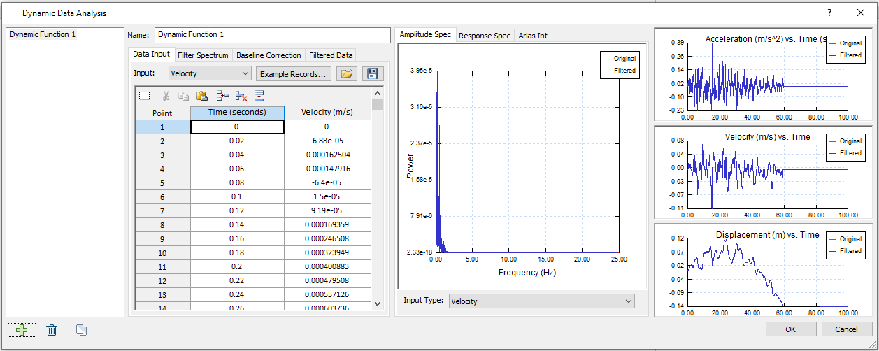
3. Select the Data Input tab under Dynamic Function 1, ensure the Input is Velocity.
4. For the first data point, manually enter Time (seconds) = 0, Velocity (m/s) = 0.
The first data point in the data input grid must start at time = 0 s in the order for the power spectrum to handle the data properly.
5. From the second point, in Sheet 2 “Model 1 – Velocity” of the Excel File, copy and paste the Time data (Column A), and the Velocity data (Column B) into the Dynamic Data Analysis dialog.
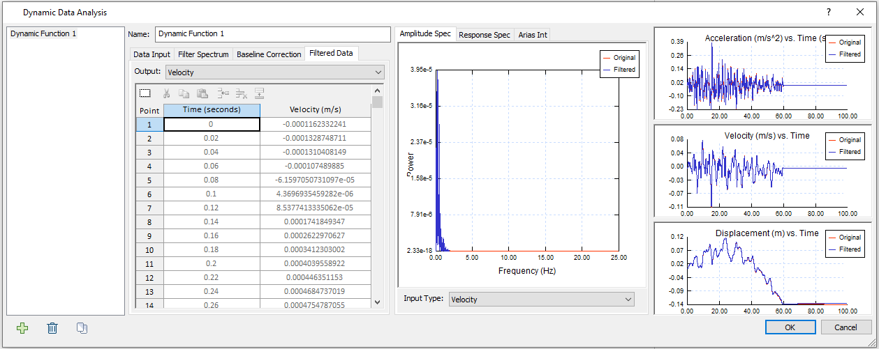
6. Make sure Input Type = Velocity under the Amplitude Spectrum tab, to show the “Power vs. Frequency (Hz)” plot based on velocity. The dialog should look as follows:
   
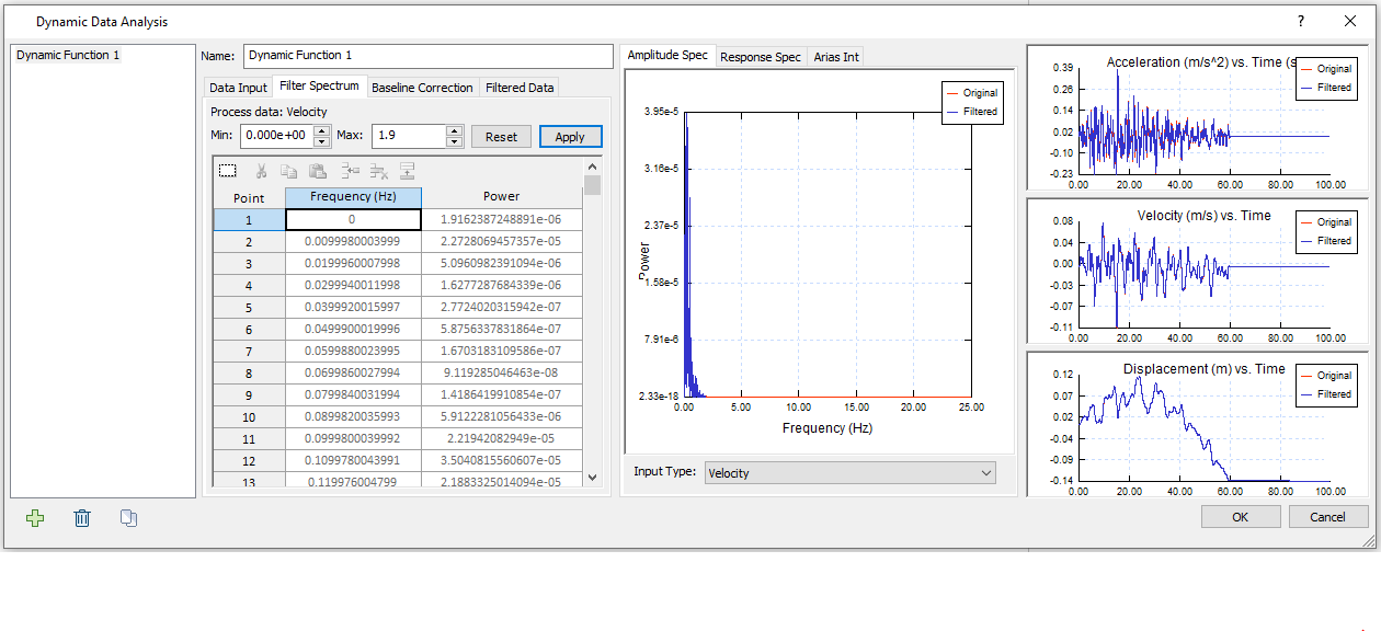
7. Select the Filter Spectrum tab. Change the Max to 1.9 Hz. Click the Apply button. The filtered Frequency vs. Power data will display below, the Power Spectrum graph will be presented to the right.
   
   
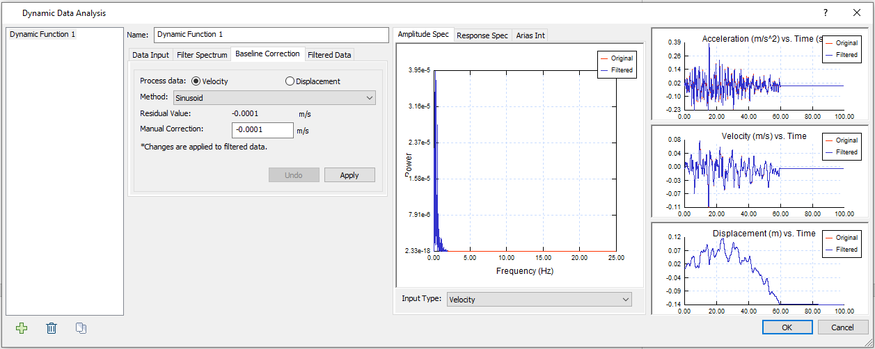
8. Select the Baseline Correction tab. Select Process data = Velocity and Method = Sinusoid. The current Residual Values is -0.0001 m/s. By default, the Manual Correction value will be the residual value. Your dialog should look as follows:
   
   
9. Click the Apply button to apply a Manual correction of -0.0001 m/s. Your dialog should now look as follows:
   
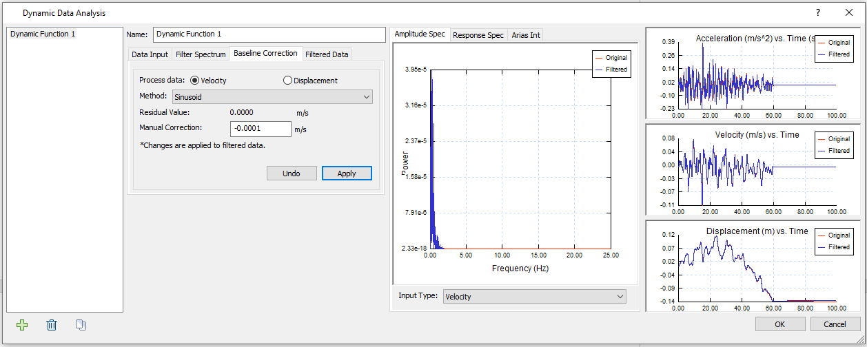
   The Residual Value is corrected to 0 m. This change is not obvious.
   
   
10. Proceed to the Filtered Data tab. The filtered velocity data is displayed below.
    
    
11. Click OK to save and close the dialog.
12. Select: Dynamic > Delete Dynamic Load
13. Select the bottom boundary and hit Enter to delete the current dynamic load.
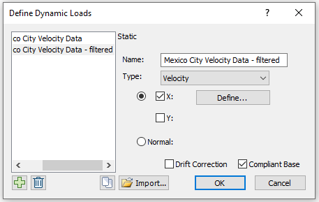
14. Select: Dynamic > Define Dynamic Loads
15. Add a new dynamic load definition. Rename “Dynamic Load 2” to “Mexico City Velocity Data - filtered”. Change the Type to Velocity and check the “Compliant Base” checkbox. Click the Define button.
    
16. In the Velocity vs. Time dialog, check the “Use filtered data” checkbox at the bottom and select Dynamic Function 1. Your dialog should look as follows:
    
    
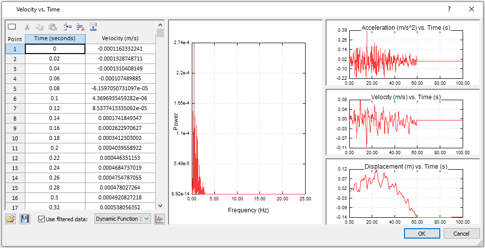
17. Click OK in the Velocity vs. Time dialog, and in the Define Dynamic Loads dialog.
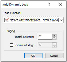
18. Select: Dynamic > Add Dynamic Load
19. Select Mexico City Velocity Data – filtered (Velocity) as the Load Function. Under the staging section, ensure Install at stage = 2. Click OK.
    
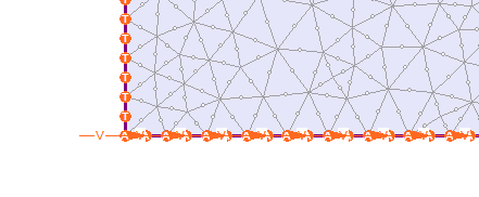
20. Using the selection tool, click on the bottom boundary and press Enter to apply the Velocity dynamic load. The boundary should look as follows:
    
    
21. Save the model as Tutorial D.
    

3.0 Results

1. Select: Analysis > Compute
2. Select: Analysis > Interpret

3.1 Stresses

Cycling through the tabs allows the user to get an idea of the stresses that are changing over time during the earthquake event.

Now switch to the second stage, labelled Intermediate 1. For dynamic nonlinear slope analysis, it is useful to plot the deformed shape and yielding elements and observe the failure over time by progressing through the stages.

1. Select: View > Display Options
2. Choose the Stress tab. Turn on the Deform Contours option.
3. Choose the Boundaries tab. Deselect the External boundary to prevent it from being displayed. Select Done to save and exit the dialog.
4. Select: Show Yield > Show Yielded Elements

Click through the different stages to see where the slope has experienced the majority of failure. Most of the failure in the slope crest is experienced by the fourth and fifth stages (Intermediate 3 and Final Stage).

3.2 Displacement

When conducting dynamic analysis, it is convenient to be able to observe the maximum displacement in the model that may occur between the stages. Beyond the time queries that were created earlier, RS2 records the maximum displacement, velocity, and acceleration observed during the simulation at each stage for all nodes. This data is used to display contours of the displacement, velocity and acceleration.

1. Turn off deformed contours from the Display Options dialog or the toolbar.
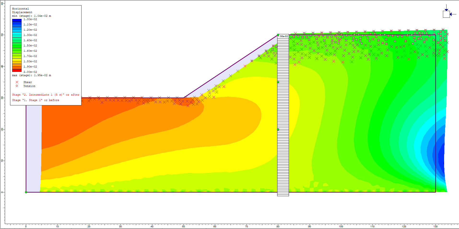
2. Use the drop-down in the toolbar to select the Dynamic > Max X Displacement dataset from the Dynamic data option.

The displacement contours demonstrate that the slope crest is moving horizontally towards to the left. It can be observed that the maximum Peak X Displacement occurs during stage three (Intermediate 2).

3. At this point, display the external boundary again using the display options or by selecting the Show/Hide External Boundary button on the toolbar.
4. Select: Query > Query Boundary.

Selecting the external boundary of the model allows the values for the peak displacement to be determined. The greatest horizontal displacement is about 0.0468 m.

The displacement time history near this observed maximum Max X Displacement can be obtained from the Time Queries that have been added.

5. Right clicking the middle Time Query point (80, 35) and selecting Graph Time Query Data will open the dynamic data graph dialog.
6. For Vertical Axis ensure X displacement is selected and click Select All to obtain the entire time history data for this point in the model.
7. Pressing the Plot button generates the time history plot.

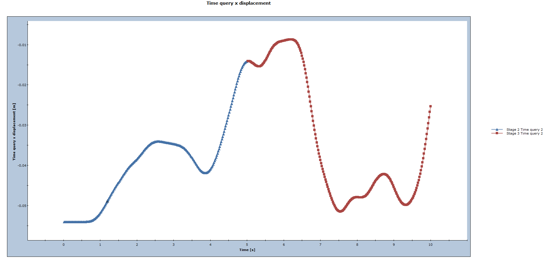
All the stages are being plotted in different colours and each time step is marked with a point marker in the time history.

Right-click in the graph space and select Peak Values > Show Peak Values to label the data point on the graph that represents the largest absolute displacement. At this point, it is 0.0451 m.

Like all graphs produced in the Interpret program, an excel spreadsheet may be produced for the user or the data can be extracted and pasted elsewhere.

8. Close the plot.

The horizontal displacement of a vertical soil profile at various stages and times may be graphed to obtain a sense of how the slope translates during the seismic event. Horizontal displacement relative to the position of the slope under gravity loading would be of greater interest since it would represent the deformation due solely to the ground excitation.

To obtain the relative motion for the dynamic stages:

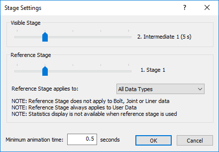
9. Select: Data > Stage Settings
10. Move the reference stage slider onto the first stage so that it reads "1. Stage 1"
11. Select OK.
    

At this point to observe the vertical profile a material query should be added.

12. Select: Query > Add Material Query
13. Enter the starting vertex of (80, 0) and another at (80, 50) and right-click and select Done.
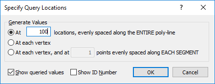
14. The Specify Query Locations dialog will open. Specify 100 as the number of locations, evenly spaced along the ENTIRE poly-line to generate values.
15. Click OK.
    
16. Use the combo box in the toolbar to select the Horizontal Displacement dataset from the Solid Displacement data option. At this point, also remove the external boundary query.
    

To obtain the plot of the vertical soil profile the following steps need to be executed.

17. Right-click on the material query poly-line and select Graph Data.
18. Select all the stages available to plot on the graph and click the Plot button.
19. The graph is generated. Select: Chart > Axes > Swap Horizontal and Vertical Axes. Swapping the axes will ensure that the horizontal displacement is on the horizontal axis.

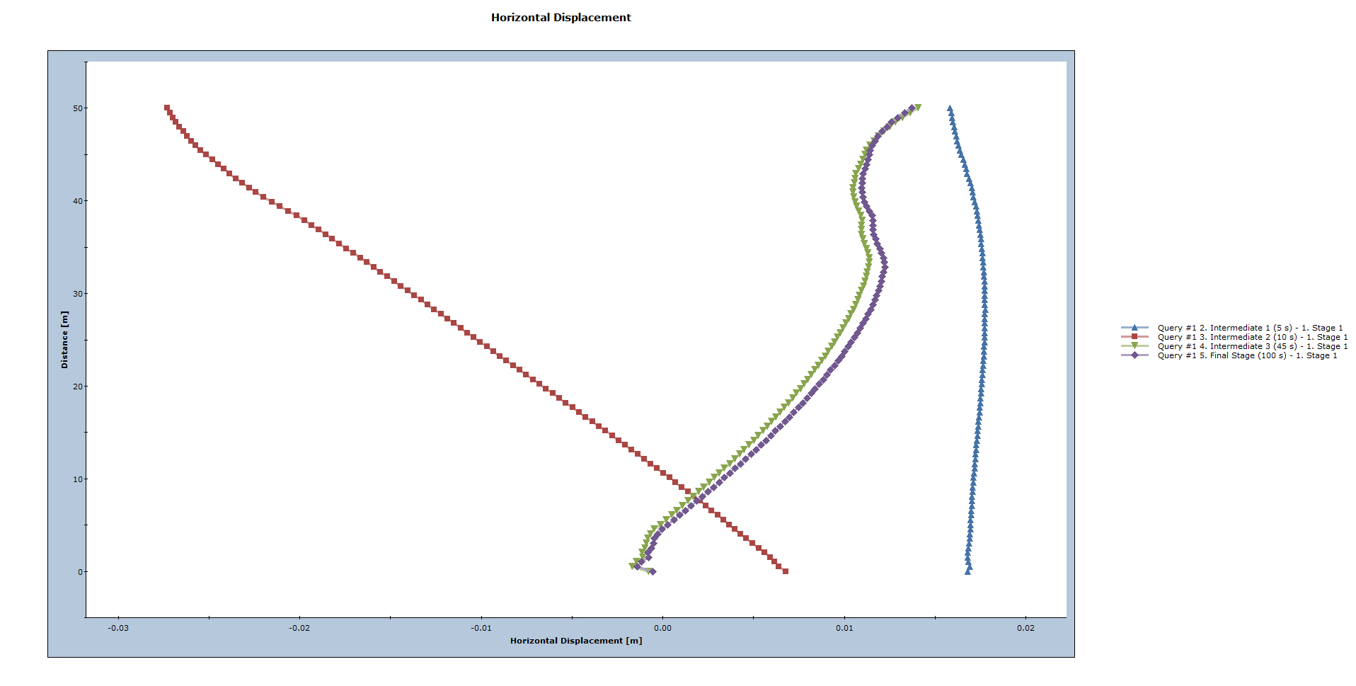
The generated plot provides an indication of how the entire slope along the depth deforms and shakes at various points during the seismic event. The greater from the vertical the plot of each stage is, the greater is the horizontal displacement at that stage. Notice that the first stage (Intermediate 1) has the least horizontal displacement.

This concludes the Dynamic Analysis Slope Part D Tutorial.