Joint Tutorial
1.0 Introduction
This tutorial involves a circular opening of 2.5-meter radius, to be excavated close to a horizontal plane of weakness (joint), located 3.5 meters above the center of the circular opening.
For this analysis, the rock mass is assumed to be elastic, but the joint will be allowed to slip, illustrating the effect of a plane of weakness on the elastic stress distribution near an opening. (This example is based on the one presented on pg. 193 of Brady and Brown, Rock Mechanics for Underground Mining, 1985 – consult this reference for further information.)
2.0 Constructing the Model
- Select Analysis > Project Settings
 or click on the icon in the toolbar to open the Project Settings dialog.
 - Ensure that the units are set to Metric, stress as MPa.
2.1 Entering Boundaries

- Select: Boundaries > Add Excavation

- Right-click the mouse and select the Circle option from the popup menu.
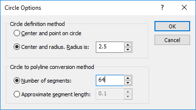
- Select the Center and radius option and enter a radius of 2.5. Enter Number of segments = 64 and select OK.
- Enter the circle center by typing 0, 0 in the prompt line. Press Enter and the circular excavation will be created.
- Select: Boundaries > Add External

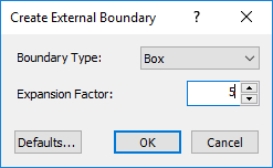
- Enter an Expansion Factor of 5 and select OK. The external boundary will be automatically created.
Now add the joint to the model.
- Select: Boundaries > Add Joint

- Click OK to accept the default settings.See the RS2 Help system for a discussion of the Joint End Condition option.
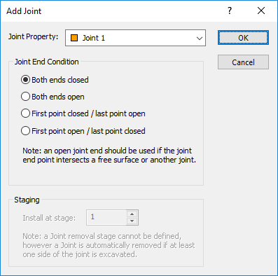
- Now enter the following coordinates defining the joint: (-30, 3.5), (30, 3.5). Press Enter.
The joint is now added to the model.
- The exact intersection of two lines is unknown.
- New vertices are required at known locations. They can be created automatically (rather than manually with the Add Vertices option).
2.2 Material Properties
![]()
The properties of the rock mass and the joint must now be entered.
- Select: Properties > Define Materials

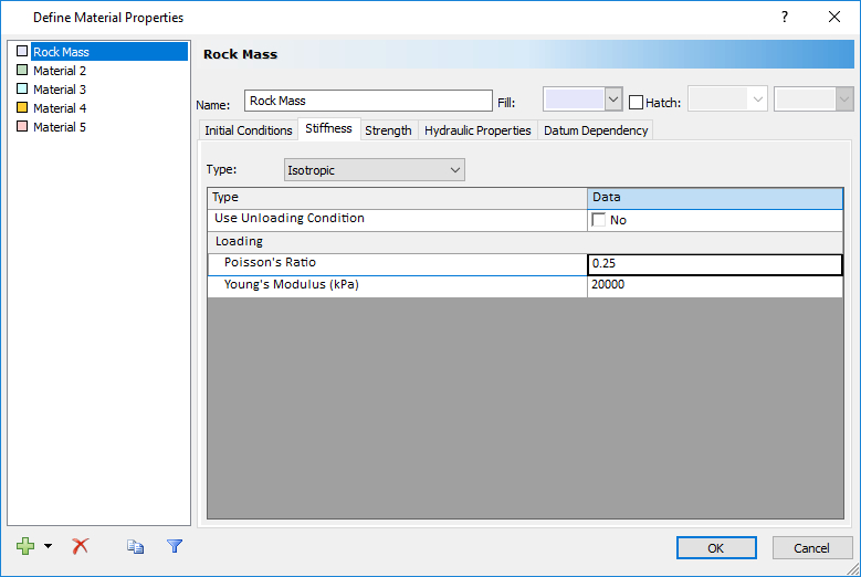
- With the first material selected in the Define Material Properties dialog, enter Name = Rock Mass. Leave the default Strength parameters. Select the Stiffness tab and enter Poisson’s ratio = 0.25. Click OK.
- Select: Properties > Define Joints

- With the first material selected in the Define Joint Properties dialog, under the Slip Criterion section, select Criterion = Mohr-Coulomb, enter Peak Frication Angle (deg) = 20.
- Under the Stiffness section, enter Normal Stiffness (MPa/m) = 250,000, Shear Stiffness = 100,000.
- Unselect the checkbox for Initial Joint Deformation. The dialog should look as follows:
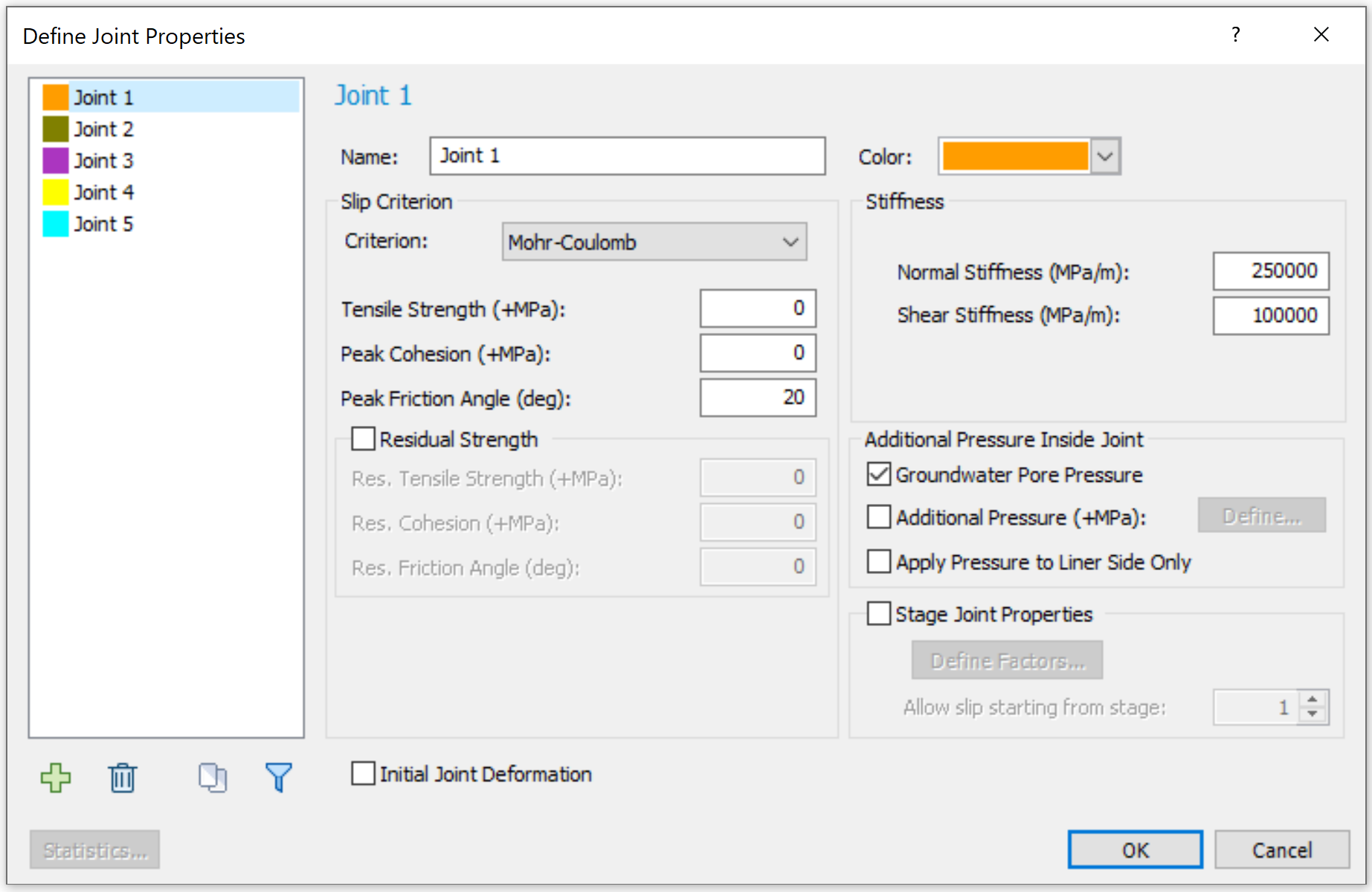
- Click OK to apply and close the dialog.
2.3 Assigning Properties
![]()
Since properties were entered for both the rock mass and the joint properties with the first material selected in the Define Properties dialogs, the properties do not need to be assigned to the model; RS2 automatically assigns the Material 1 and Joint 1 properties.
- Right-click the mouse within the circular excavation.
- In the popup menu, go to the Assign Materials sub-menu, and select the Excavate option.
2.4 Field Stress
![]()
- Select: Loading > Field Stress
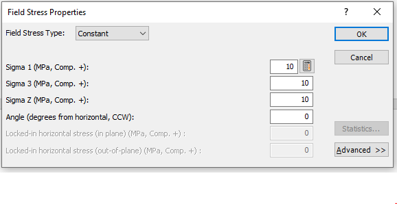
- In the Field Stress Properties dialog, select Field Stress Type = Constant and ensure Sigma 1, 3 and Z are set to 10 MPa.
- Click OK.
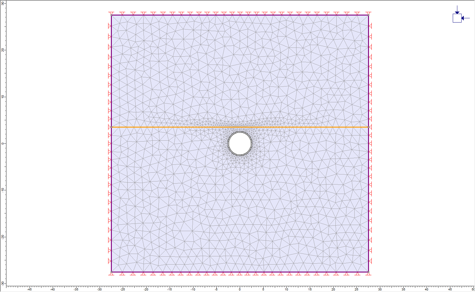
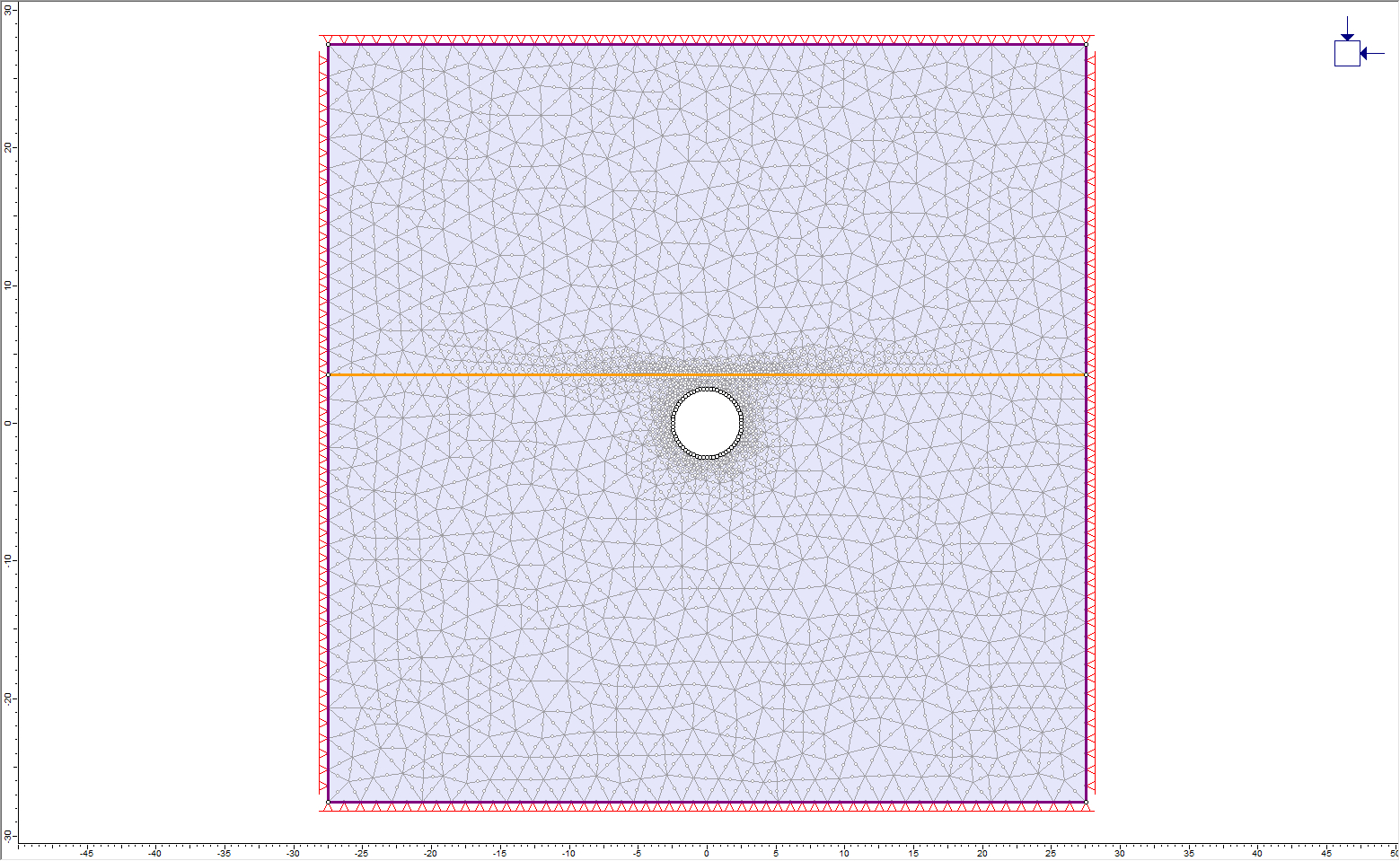
2.5 Mesh

- Select: Mesh > Mesh Setup

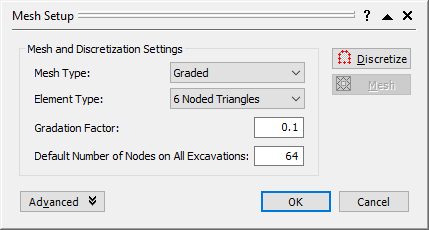
- In the Mesh Setup dialog, enter Number of Excavation Nodes = 64. Click OK.
- Select: Mesh > Discretize and Mesh

The finished model should appear as below:
3.0 Compute
- Select: Analysis > Compute

4.0 Results and Discussion
- Select: Analysis > Interpret

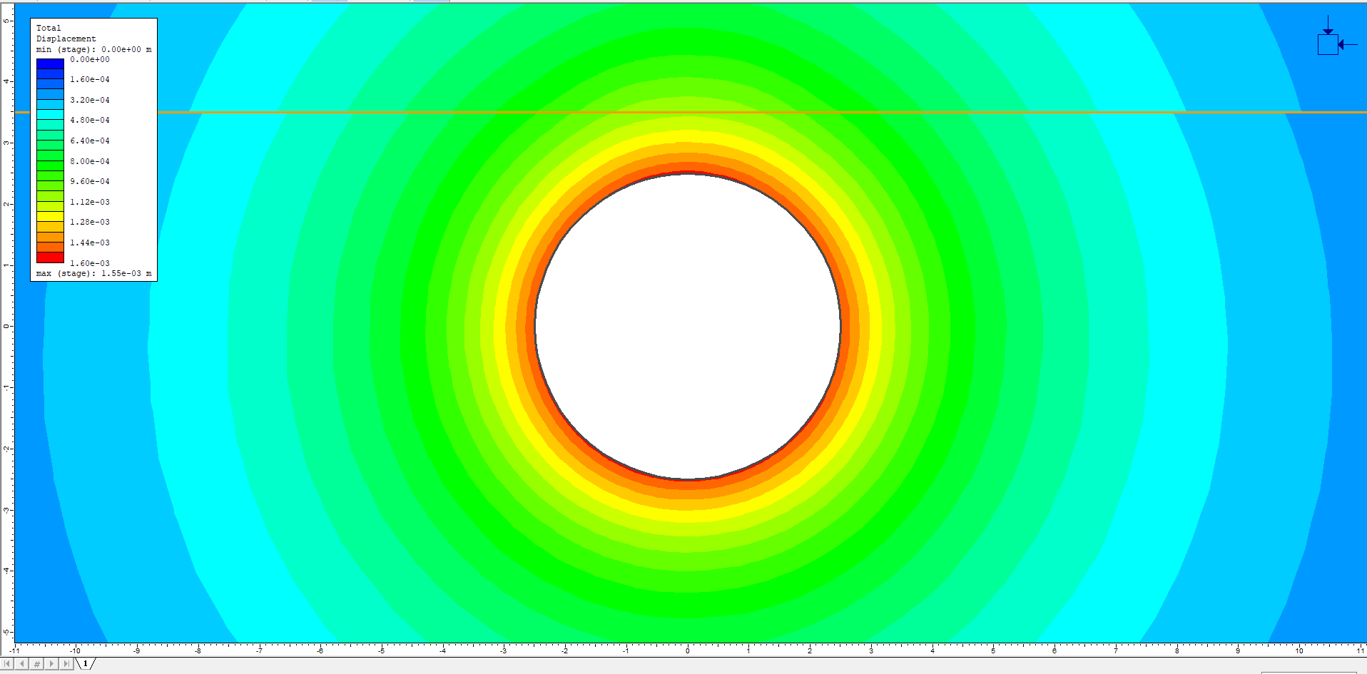
Let’s zoom in so that we can get a better look at what’s going on near the excavation.
- Click the Zoom Excavation
 button on the toolbar.
 - Press F4 three times to zoom out.
Observe the effect of the joint on the Sigma 1 contours. Notice the discontinuity of the contours above and below the joint. The effect of the joint is to deflect and concentrate stress in the region between the excavation and the joint.
- Select Total Displacement from the drop-down menu in the toolbar to view total displacement contours.
The discontinuity of the displacement contours may not be immediately apparent.
- In the Contour Options dialog, turn on the Filled (with Lines) contour mode so that the discontinuity of the displacement contours can be more easily seen.
4.1 Joint Yielding
Now let’s check for yielding of the joint.
- Turn on the display of yielded elements and yielded joints

The yielded joint elements are highlighted in red on the model, and the number of yielded elements is displayed in the status bar: 15 yielded joint elements
Two separate zones of yielding in the joint can be seen, to the right and left of the excavation. Notice that the region of joint slip corresponds to the region of contour discontinuity, above and below the joint.
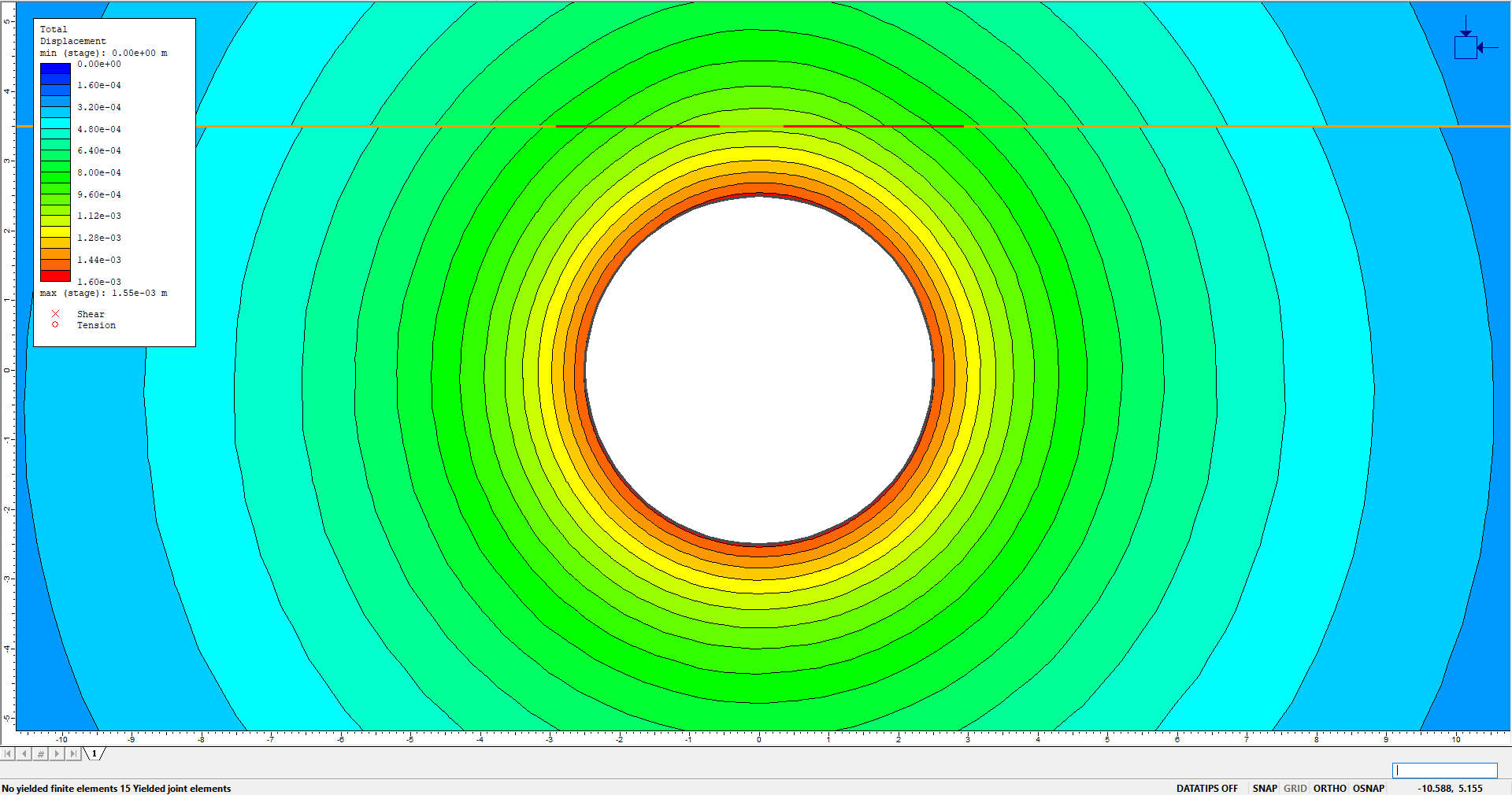
- In the Contour Options dialog, change the contour mode from Filled (with Lines) to Filled.
4.2 Graphing Joint Data
Graphs of normal stress, shear stress, normal displacement and shear displacement can be easily obtained for joints, using the Graph Joint Data option.
- Select: Graph > Graph Joint Data

Since there is only one joint in the model, it is automatically selected. In the Graph Joint Data dialog: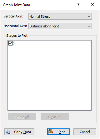
- Select Plot to generate a plot of Normal Stress along the length of the joint.
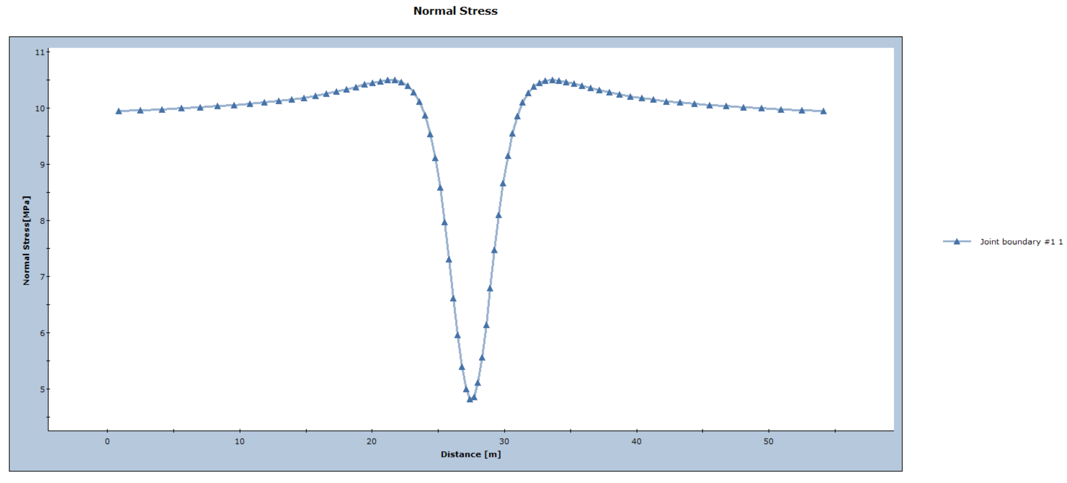
As expected, there is a sharp drop in normal stress where the joint passes over the excavation.
- Now, repeat the above procedure to create a graph of shear stress along the joint. In the Graph Joint Data dialog:
- Plot Vertical Axis as Shear Stress
- Plot Horizontal Axis as Distance along joint
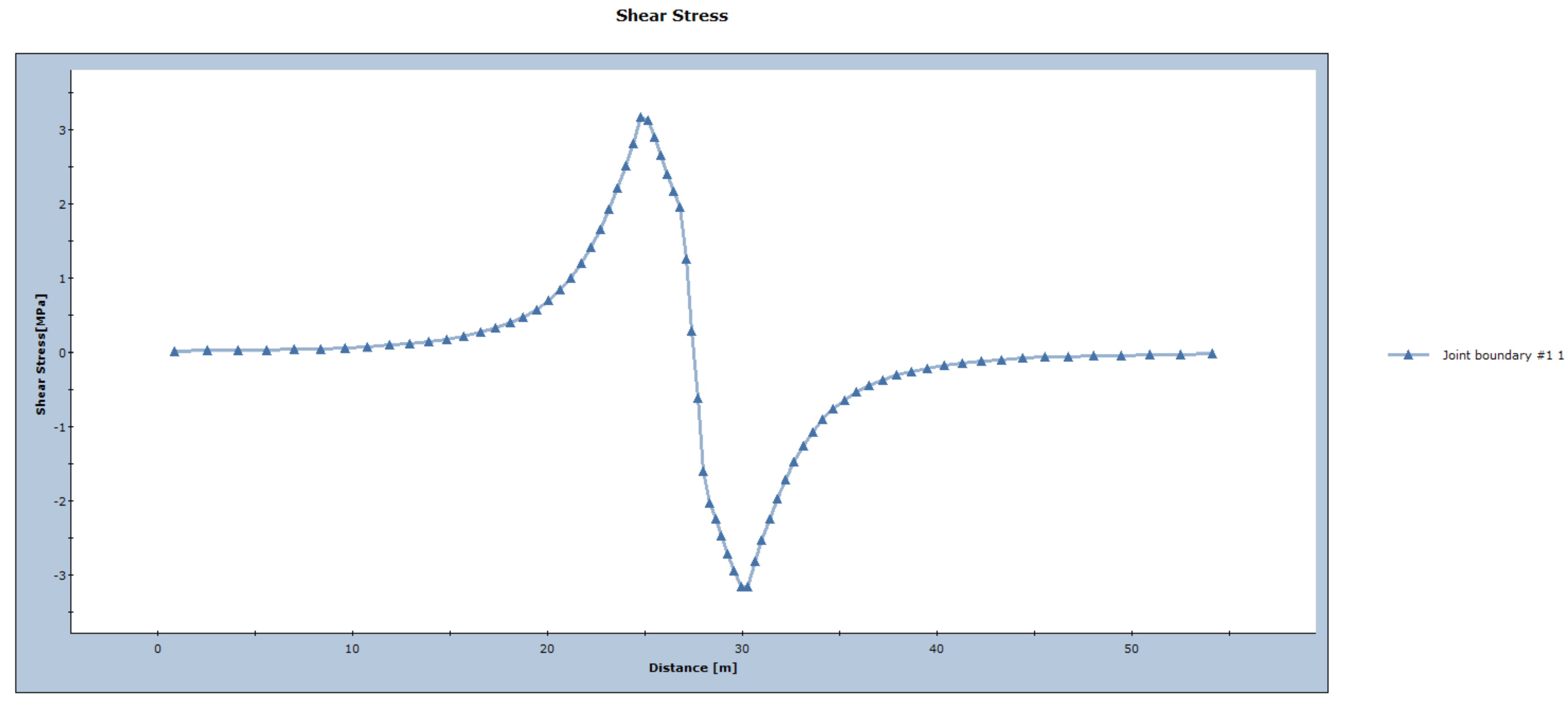
Notice the reversal of the shear stress direction over the excavation. It is this sense of slip which produces the inward displacement of rock on the underside of the plane of weakness.
4.3 Critical Friction Angle for Slip
Calculations in Brady & Brown indicate that if the angle of friction for the plane of weakness exceeds about 24-degrees, no-slip is predicted on the plane, and the elastic stress distribution can be maintained. Run the analysis using angles of friction for the joint of 20 to 24 degrees, then use the Yielded Joints option (as described above) to check the slip on the joint. Results should appear as below:
| Angle of friction for joint | Number of yielded joint elements |
| 20° | 15 |
| 21° | 12 |
| 22° | 9 |
| 23° | 5 |
| 24° | 0 |
These results confirm that the critical angle for joint slip in this example is around 24 degrees.
5.0 References
Brady, B.H.G. and Brown, E.T., Rock Mechanics for Underground Mining, George Allen & Unwin, London, 1985, pp193-194.