Dynamic Slope Analysis B

Filtering the Input Velocity of Seismic Loading

1.0 Introduction

When modeling seismic loading, both the frequency content of the input wave and the wave speed of the system will affect the numerical accuracy of wave transmission. Kuhlemeyer and Lysmer (1973) show that for the accurate representation of wave transmission through a model, the spatial element size should be:

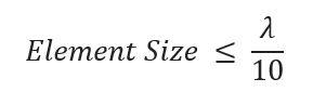
where is the wave length associated with the highest frequency component that contains appreciable energy. To satisfy the Kuhlemyer and Lysmer (1973) for a velocity input with high peak and short rise time, a very fine mesh may be required. This may lead to an excessive amount of computing time. Fortunately, for most earthquakes, the greater part of the power of the input velocity is contained in the lower-frequency components. By filtering the input velocity and removing high-frequency components, a coarser mesh may be used without significantly affecting the results. This tutorial outlines the procedure for filtering the frequencies of the input wave without losing a significant proportion of the earthquake’s power.

2.0 Constructing the Model

2.1 Project Settings

1. Select: Analysis > Project Settings
2. Under the General page, define the units as being “Metric, stress as kPa”. For this tutorial the Time Units need to be specified as "Seconds".
   
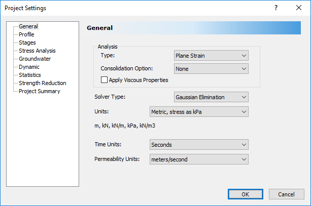
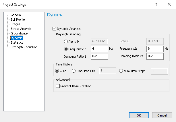
3. Select the Dynamic page. Check the Dynamic Analysis check box to enable the dynamic analysis to be conducted on specific stages. On this tab, the general dynamic parameters are defined (e.g. Rayleigh Damping).
   
   Soil systems can have damping ratio values ranging from 10% to over 20% of critical damping. For this analysis the model will be damped at 20% critical damping for the frequencies 4 and 8 Hz.
   
4. Check the Frequency1 radio button and enter 4 and 8 Hz for the frequencies and 0.2 for both Damping ratios. The remaining parameters are left at their default values.
   
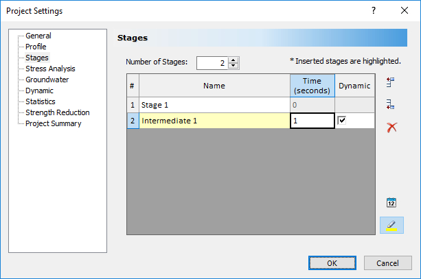
   In addition to an initial static stage, a dynamic stage will be added to see the final state of the model. The earthquake acceleration history has a duration of 60 seconds, but this tutorial only examines the intermediate stage after 1 second.
   
5. Select the Stages page. The first stage in the analysis is, by default, always a static analysis stage. Insert a new stage and check the Dynamic check box. In the time column the simulation time at which each stage will end is inserted. Change the time of the second stage to 2 seconds. Rename the second stage “Intermediate 1.”
   
   
6. Select the Stress Analysis page. Ensure the Convergence Type is set to Comprehensive. Make sure the Number of Load Steps is entered as “Auto”.
7. “Accelerate initial stiffness” should be checked, with a Min Alpha of 0.2 and a Max Alpha of 5.
   
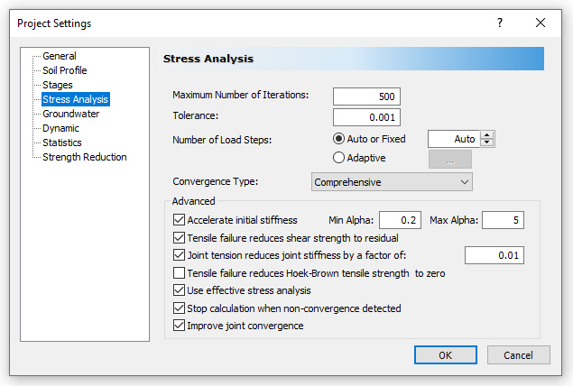
8. Leave other settings as default. Your dialog should look the same as the figures shown above.
9. Close the Project Settings dialog by pressing the OK button.

2.2 Boundaries

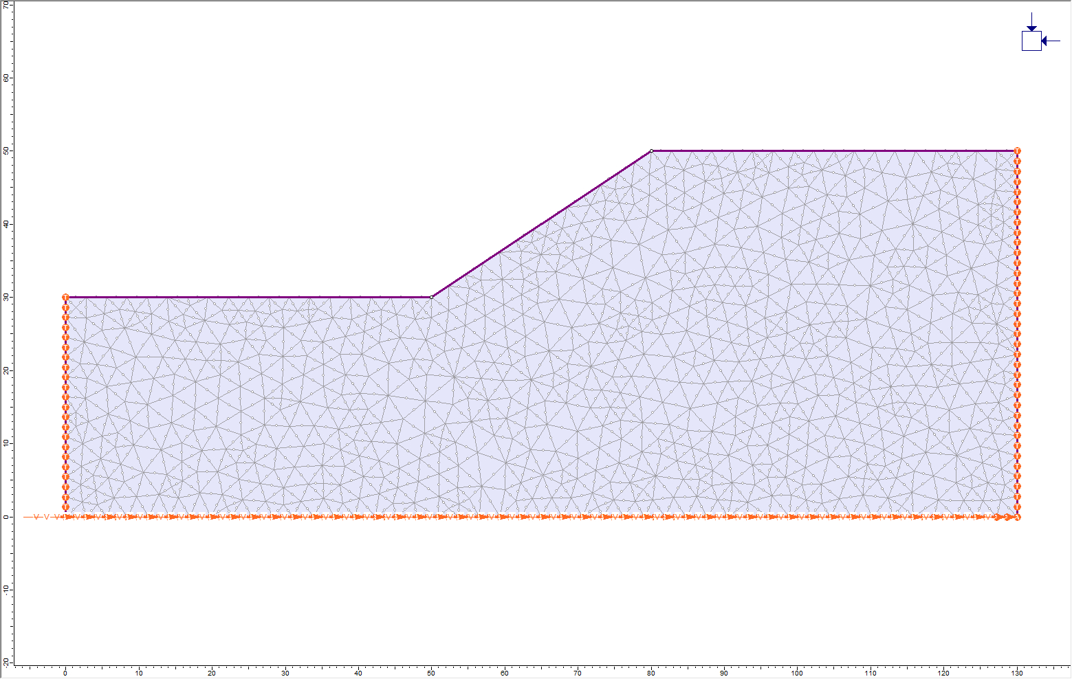
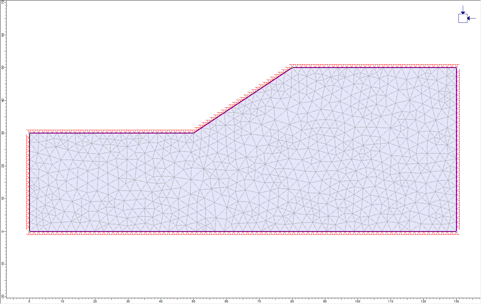
This model only requires an External boundary to define the geometry.

1. Select: Boundaries > Add External
2. Enter the following coordinates: (130, 0), (130, 50), (80, 50), (50, 30), (0, 30), (0, 0), and press “c” to close the boundary.

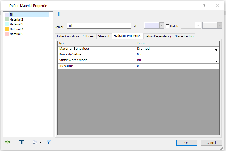
2.3 Material Properties

Define the material properties of the soil that comprises the slope.

1. Select: Properties > Define Materials
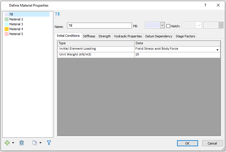
2. Select the Initial Conditions tab. Change the name of Material 1 to “Till.” Ensure the Initial Element Loading is set to Field Stress & Body Force (both in-situ stress and material self-weight are applied). Enter a Unit Weight of 19 kN/m3.
   
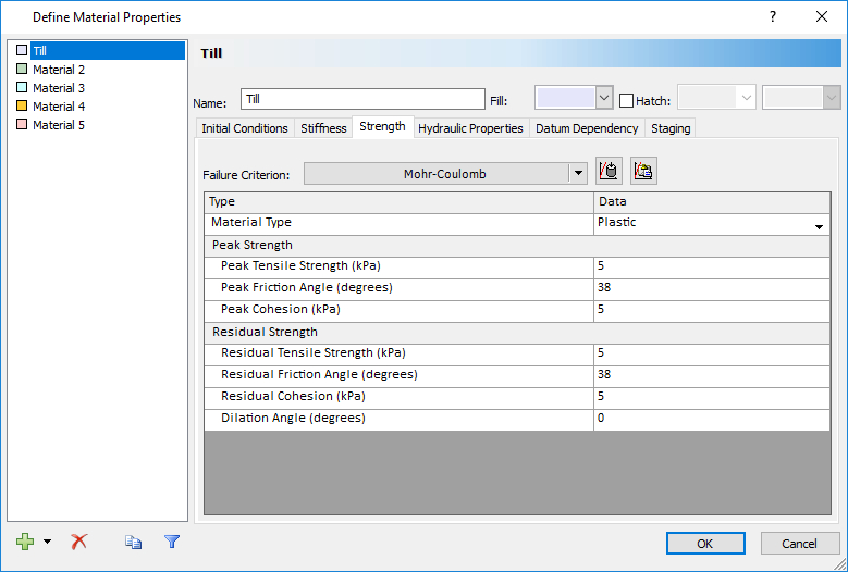
3. Select the Strength tab and make sure the Failure Criterion is set to Mohr-Coulomb.
   
• Set the Material Type to Plastic, meaning the material can yield/fail. Set the peak and Residual Tensile Strength to 5 kPa.
• Set the peak and residual cohesion to 5 kPa.
• Set the peak and residual friction angle to 38°. Leave the dilation angle at 0° (no volume increase when sheared, non-associated flow rule).



4. For Elastic Properties, select the Stiffness tab.
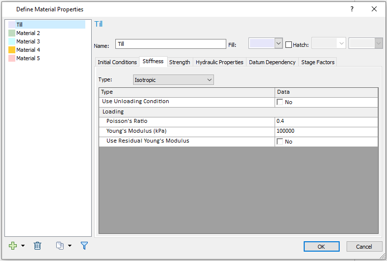
• Enter 0.4 for the Poisson ratio and 100 000 kPa for the Young’s Modulus.



5. Select the Hydraulic Properties tab. Set the Static Water Mode to Ru and leave the Ru Value as 0.



6. Press the OK button to save properties and close the dialog.

2.4 Loading

1. Select: Loading > Field Stress
2. In the Field Stress Properties dialog, change the Field Stress Type to Constant. Your dialog should look as follows:
   
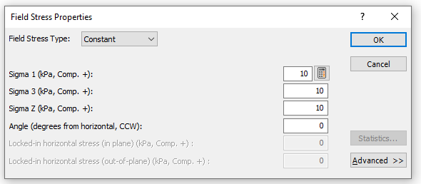
3. Click OK to close the dialog.
   

2.5 Mesh

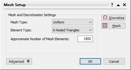
Now, generate the finite element mesh. First, its necessary to define the parameters (type of mesh, number of elements, type of element) used in the meshing process.

1. Select: Mesh > Mesh Setup
2. In the Mesh Setup dialog, change the Mesh Type to Uniform, the Element Type to 6 Noded Triangles, and the number of elements to 1500.
3. Close the Mesh Setup dialog by selecting the OK button.
   
4. Select: Mesh > Discretize and Mesh

2.6 Boundary Conditions (External)

The portion of the external boundary representing the ground surface (0,30 to 50,30 to 80,50 to 130,50) must be free to move in any direction.

1. Select: Displacements > Free
2. Use the mouse to select the three line segments defining the ground surface of the slope.
3. Right-click and select Done Selection.

For this analysis, the lateral boundaries will be allowed to move vertically and only be restrained in the horizontal direction in Stage 1. In Stage 2, all restraints will be removed.

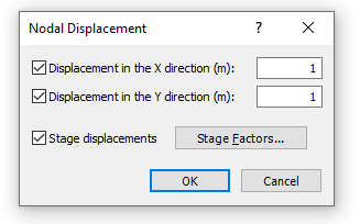
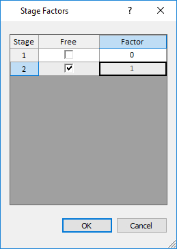
4. Select: Displacements > Set Displacement
   
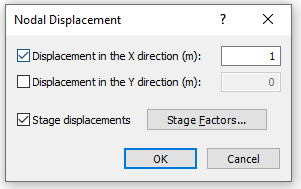
5. Enter Displacement in X direction = 1 and uncheck the Displacement in Y direction check box.
6. Check the “Stage displacements” box and click on the Stage Factors button.
7. In the dialog, change the factor of Stage 1 to zero. Check the Free box for Stage 2.

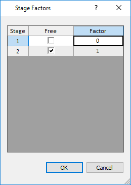
A factor of zero represents a zero-displacement boundary condition. The free check box means that the nodes in Stage 2 are free to move without restraint. A factor of 1 means that the displacement will be equal to the magnitude(s) entered in the Nodal Displacement dialog.

Therefore, all lateral restraints were removed in the second stage and a zero-displacement boundary set in the x direction condition in Stage 1.

8. Select OK in the Stage Factors dialog and select OK in the Nodal Displacement dialog.
9. Using the resulting selection tool, click on the lateral boundaries and press Enter.

To free the bottom boundary:

10. Select: Displacements > Set Displacement
11. Enter Displacement in X direction = Displacement in Y direction = 1.
12. Check the “Stage displacements” box and click on the Stage Factors button.
    
13. In the dialog, change the factor of Stage 1 to zero. Check the Free box for Stage 2.
    
    
14. Select OK in the Stage Factors dialog and select OK in the Nodal Displacement dialog.
15. Using the resulting selection tool, click on the bottom boundary and press Enter.

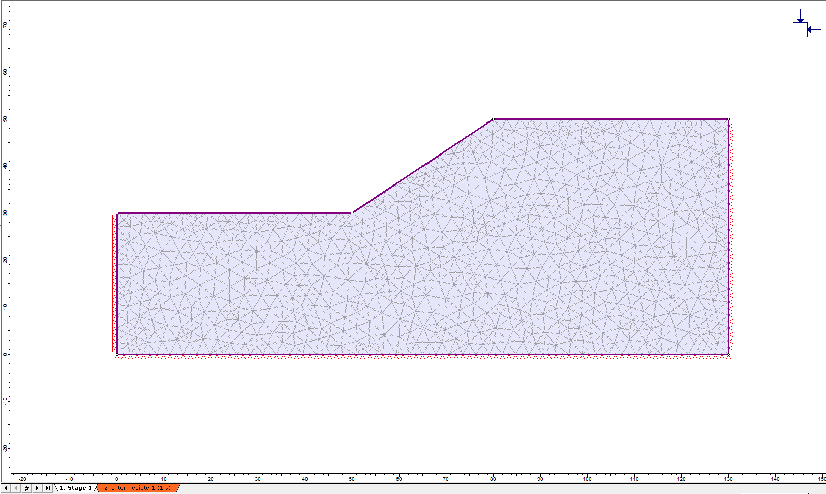
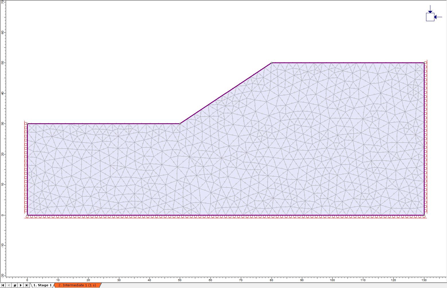
In Stage 1, the displacement boundary conditions should appear as follows.

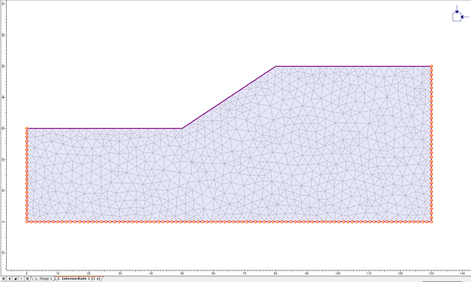
Now click on the Intermediate 1 tab at the bottom left of the window. Notice that Intermediate 1 has no restraints, as defined.

2.7 Boundary Conditions

Let’s assign dynamic boundary conditions to the boundaries of the model.

1. Ensure that the second stage of the Dynamic workflow tab is selected. Right-click on one of the lateral sides of the model and select Set Transmit BC. Do this for both lateral sides of the column.
2. Right-click on the bottom boundary and select Set Absorb BC.
   
3. Save the model using the Save option in the File menu.
   

3.0 Results and Discussion

Looking at the mesh, pick out an element that appears to have a very long dimension.

1. Select: Tools > Dimension Length to display an approximate maximum element length, as shown.

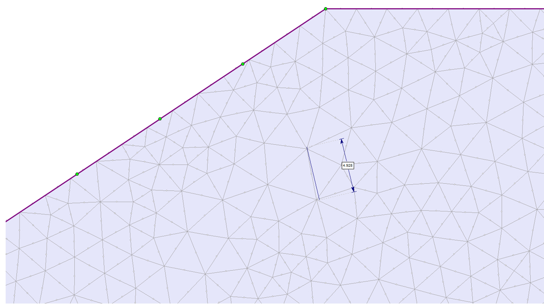
A maximum dimension of 4.928 m will be used. Therefore, the minimum wave length should be approximately:

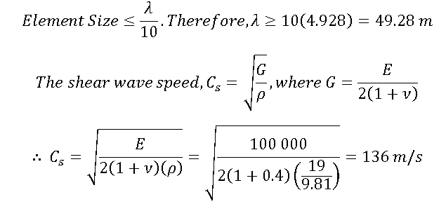
The maximum frequency that still maintains the accuracy of the model is:

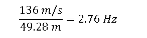
This maximum frequency will be used to filter the spectrum. Using a value of around 2.8 Hz will not result in noticeable changes. For tutorial purposes, we will use a value of 1.9 Hz for filtering which corresponds to using a Young’s Modulus of 50 000 kPa.

Let’s input the earthquake data for the 1985 Mexico City earthquake as a dynamic load. This data can be found in Sheet 2 of the Excel Sheet in the installation folder. For Windows 7 and 8 the file path is:

C:\Users\Public\Documents\Rocscience\RS2 Examples\tutorials\Dynamic Analysis\Dynamic Slope Analysis

1. Open the Excel file titled “Mexico City 1985 - Mesa Bivradora C. U.”
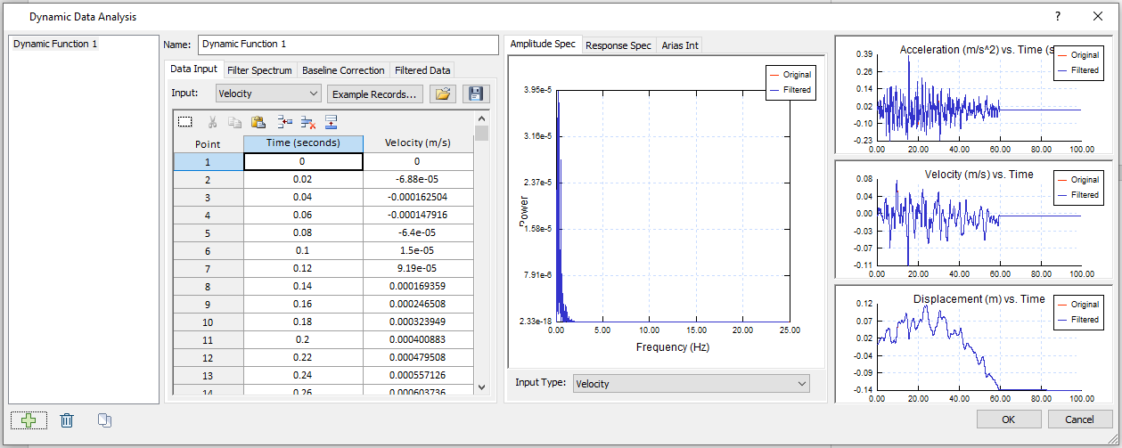
2. Select: Dynamic > Dynamic Data Analysis
3. Select the Data Input tab under Dynamic Function 1, ensure the Input is Velocity.
4. For the first data point, manually enter Time (seconds) = 0, Velocity (m/s) = 0.
Note: The first data point in the data input grid must start at time = 0 s in the order for the power spectrum to handle the data properly.
5. From the second point, in Sheet 2 “Model 1 – Velocity” of the Excel File, copy and paste the Time data (from cell A5 to A5004), and the Velocity data (from cell B5 to B5004) into the Dynamic Data Analysis dialog.
6. Make sure under the Amplitude Spectrum tab in the middle section of the dialog, Velocity is selected as input type to show the “Power vs. Frequency (Hz)” plot base on velocity. The dialog should look as follows:
   
7. Select the Filter Spectrum tab. Enter Max = 1.9 Hz and click the “Apply” button to the right.
   
   The two columns display the Frequency (Hz) vs. Power data within the defined range. We can see from the plot, that most of the power of the earthquake occurs for frequencies of about 1.9 Hz and below. Therefore, we can filter out the other frequencies. Your dialog should look as follows: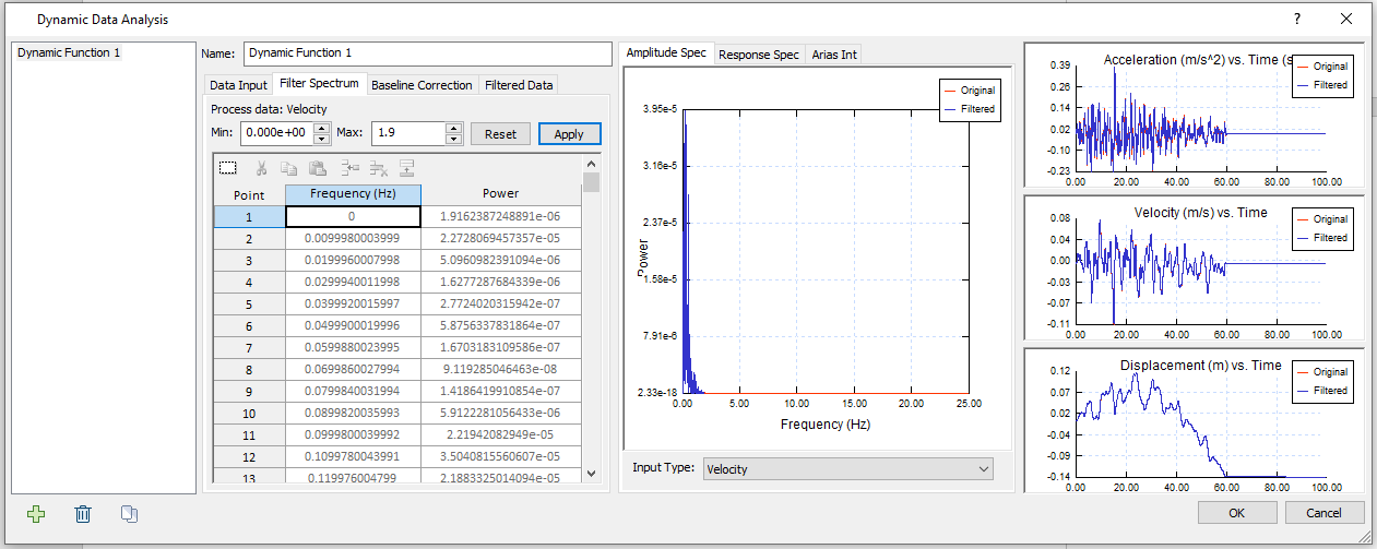
   
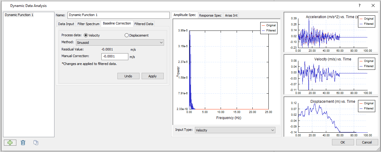
8. Select the Baseline Correction tab. Select Process data = Velocity, and Method = Sinusoid. The current Residual Value is displayed as -0.0001 m/s. This value is put in Manual Correction. Your dialog should look as follows:
   
   
9. Click Apply. Now the baseline has been corrected as follows:
   
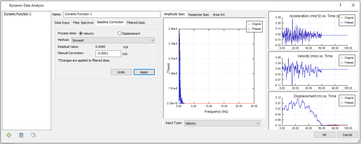
   The residual value changes to 0 m/s. No significant loss was observed from the plots. It means that the input data had been corrected sufficiently.
10. Select the Filtered Data tab. The filtered data are displayed, and the data type can be selected with the Output dropdown bar. We will apply velocity output to the model.
    
    
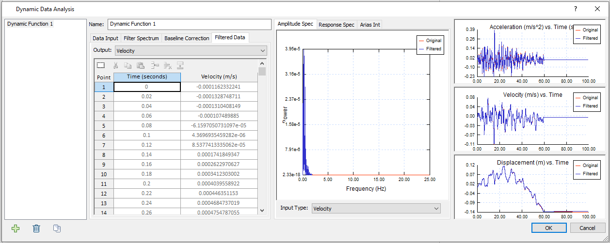
11. Click OK to save the data and close the dialog.
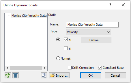
12. Select: Dynamic > Define Dynamic Loads
13. Rename “Dynamic Load 1” to “Mexico City Velocity Data.” Change the Type to Velocity and check the “Compliant Base” check box. Your dialog should look as follows:
    
14. Click the Define button.
15. In the Velocity vs. Time dialog, check the “Use filtered data” checkbox at the bottom. Select “Dynamic Function 1”. The filtered velocity data we just defined will be inputted. Your dialog should look as follows:
    
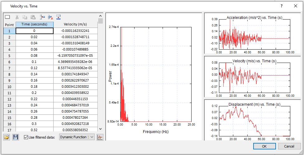
16. Click OK to save and close the Velocity vs. Time dialog. Click OK again to exit the Define Dynamic Loads dialog.
    
17. Select: Dynamic > Add Dynamic Load
• In the Add Dynamic Load dialog, the Load Function should be the dynamic load we have just defined, installed at stage 2. Click OK.
• Using the selection tool, click on the bottom boundary and press Enter.
18. Select: Dynamic > Time Query > Add Solid Time History Query
19. Enter coordinates (80, 50). Hit Enter to place the time query point. Hit Enter again to exit.
20. Select: File > Save As
21. Save the model as “Dynamic Slope Analysis Part B (After filtering)”.
22. Select: Analysis > Compute

It will be left as an exercise for the user to graph the resulting velocity at a query point and compare the difference in results.

The before filtering model is given under below. The input dynamic data is without filtering frequencies greater than 1.9 Hz.

File > Recent Folders > Tutorial Folder > Dynamic Slope Analysis Part B (Before filtering).fez

The following graph represents the velocity at a query point located at (80, 50), before and after filtering:

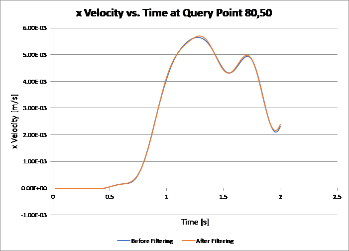
The velocity data does not change very much after filtering. Therefore, by filtering out frequencies larger than 1.9 Hz, an accurate wave transmission through the model has been obtained without losing any significant earthquake power.

This concludes the Dynamic Slope Analysis Part B Tutorial.

4.0 References

Kuhlemeyer, R.L and Lysmer, J. (1973) Finite element method accuracy for wave propagation problems. Journal of Soil Mechanics and Foundation Division. 99:5 (421-427)