Anchored Sheet Pile Wall
1.0 Introduction
This tutorial illustrates a practical application of RS2 Scripting. The RS2 Scripting feature is an API tool based on the Python programming language, designed to model and interpret results with the interface.
The model in the tutorial is the same as in the Anchored Sheet Pile Wall tutorial. Instead of construction and support features, here we will focus on the workflow automation and extended analysis capabilities with RS2 Scripting.
The RS2 Scripting functionalities covered in this tutorial include:
- Manage files through Open, Close, Save and Compute
- Modify property values of materials and supports (i.e., joints, liners, and bolts)
- Interpret contour data by stage
- Add and extract material queries
- Extract liner results
- Import/Export CSV files
Before proceeding with the tutorial, make sure you’ve gone through Getting Started with RS2 Python Scripting tutorial so you have initial setup with RS2 Scripting completed.
Tutorial Files
All tutorial files installed with RS2 can be accessed by selecting File > Recent > Tutorial Folder from the RS2 main menu. The starting files can be found in the Scripting > Anchored Sheet Pile Wall subfolder, including an initial model file, a python file, a required library list text file, and four csv files of input data for material, joints, liner, and bolts respectively. A final model file can be found in the Scripting > Anchored Sheet Pile Wall > results subfolder. During the tutorial, more output files will be generated and stored under results subfolder.
2.0 Open RocScript Editor
Launch the RocScript Editor and open anchored_sheet_pile_wall.py python file.
- Open the RS2 Modeler program.
- Select Scripting > Open Scripting Editor from the top menu. The RocScript Editor (VSCodium) will be launched.
- In the RocScript Editor, select File > Open Folder, and select folder C:\Users\Public\Documents\Rocscience\RS2 Examples\Tutorials\Scripting\Anchored Sheet Pile Wall.
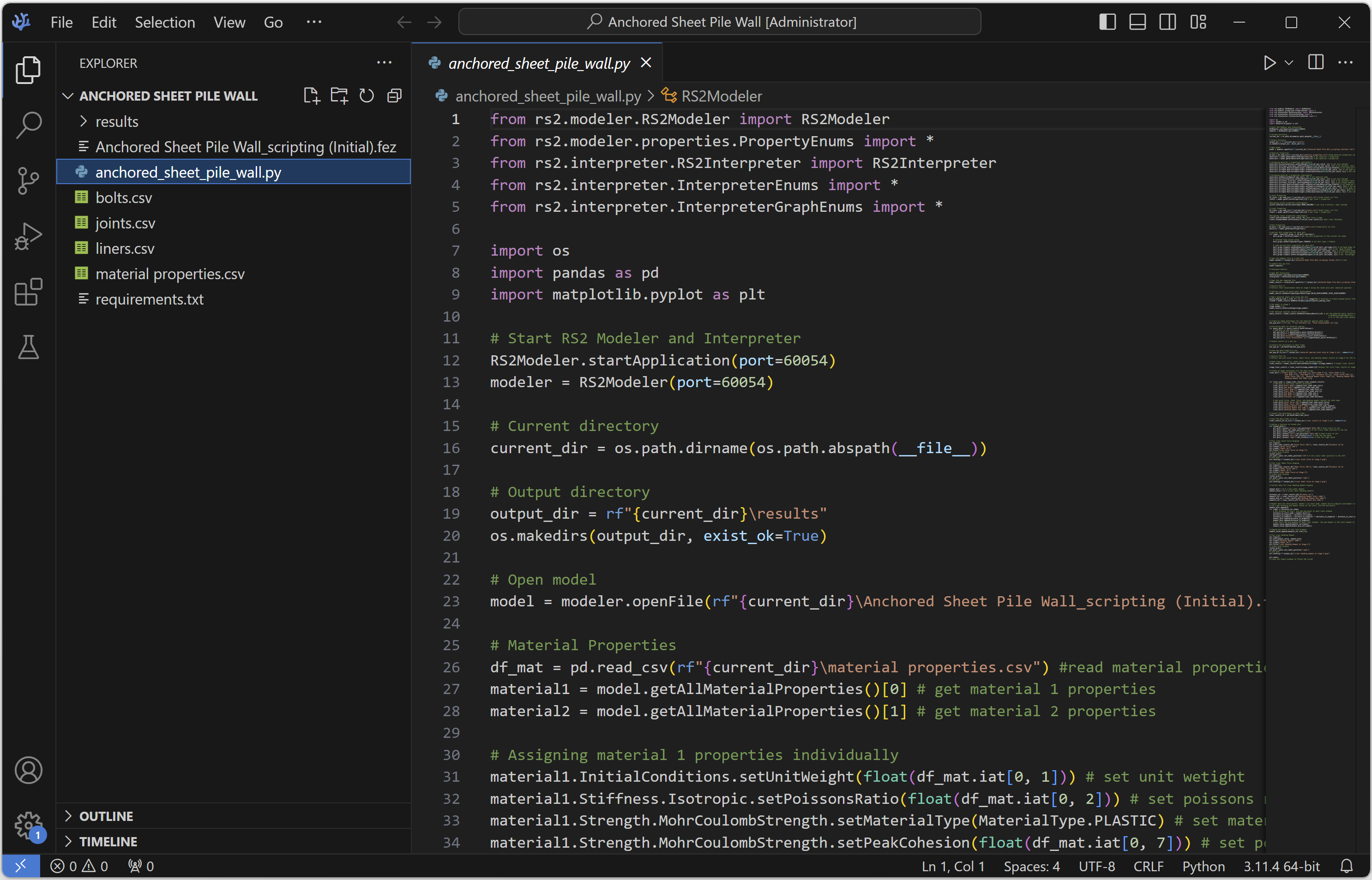
- Navigate to the Explorer tab on the left, select anchored_sheet_pile_wall.py from the list. The file will be displayed as shown below.
2.1 Install Libraries
The RS2 Python API Library is required for RS2 Scripting. It is an open-source library designed to interact with RS2 through Python. In this tutorial, we’ll also use two additional popular Python libraries:
- Pandas – for data structuring and analysis
- Matplotlib – for graphing data.
All three libraries come pre-installed with the RocScript Editor within the RS2 package. No manual installation is needed.
Advanced Users
For advanced users who are using their own python environment, you will need to install required libraries manually.
- Run the following command in your own terminal or command prompt:
Pip install -r requirements.txt
The requirements.txt file lists out the above-mentioned libraries. The file can be found in the tutorial folder.
3.0 Starting the Script
3.1 Import required modules
Import the required modules from RS2 Python API library, pandas, and matplotlib library.
from rs2.modeler.RS2Modeler import RS2Modeler
from rs2.modeler.properties.PropertyEnums import *
from rs2.interpreter.RS2Interpreter import RS2Interpreter
from rs2.interpreter.InterpreterEnums import *
from rs2.interpreter.InterpreterGraphEnums import *

import os
import pandas as pd
import matplotlib.pyplot as plt
3.2 Start the RS2 Modeler
The .startApplication() method starts an application on a server with a specified port number.
The call RS2Modeler.startApplication(port=60054) starts the RS2 Modeler, and it also starts a server on port 60054 at the same time. This action is equivalent to manually opening the RS2 Modeler, and navigating to the Manage Scripting Server option from the Scripting menu, setting port number to 60054 and clicking Start Server (see more of the options).
# Start RS2 Modeler
RS2Modeler.startApplication(port=60054)
modeler = RS2Modeler(port=60054)
3.3 Organize Directories
Extract the current file directory.
# Current directory
current_dir = os.path.dirname(os.path.abspath(__file__))
Inside the current directory, create (or use – if there exists one) a folder named “results” to store result files.
# Output directory
output_dir = rf"{current_dir}\results"
os.makedirs(output_dir, exist_ok=True)
4.0 Constructing the model
- Open the initial model file Anchored Sheet Pile Wall_scripting (Initial).fez in RS2 Modeler.
For the initial model, the model construction (including project settings, geometry, staging, loading, field stress, mesh, and boundary conditions) has been completed, except for the material and support properties are at their default values. We need to define the material, joint, liner, and bolt properties before computing the model.
# Open model
model = modeler.openFile(rf"{current_dir}\Anchored Sheet Pile Wall_scripting (Initial).fez")
4.1 Define Material Properties
Now, we will modify the material properties using data from a CSV file.
4.1.1 Import CSV file
We import data from the material properties.csv file, which can be found in the current directory.
# Material Properties
df_mat = pd.read_csv(rf"{current_dir}\material properties.csv") #read material properties csv file
Get current Material 1 and Material 2 properties in the model.
material1 = model.getAllMaterialProperties()[0] # get material 1 properties
material2 = model.getAllMaterialProperties()[1] # get material 2 properties
4.1.2 Assign Material Properties
Assign material properties from CSV data to the model.
- For Material 1, we need to modify the following:
- Unit Weight = 17
- Poisson’s Ratio = 0.25
- Material Type = Plastic
- Peak Cohesion = 1
- Residual Cohesion = 1.
Code Explain:
The pd.read_csv() method loads the CSV into a DataFrame.
Example: For the data below:
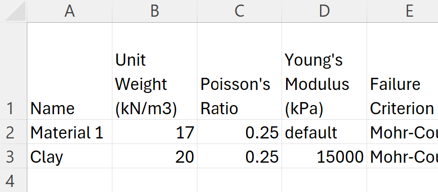
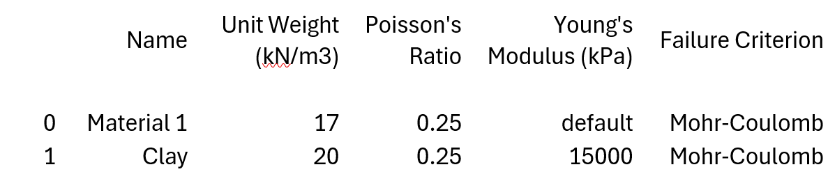
The resulted DataFrame will be:
For more information about a DataFrame structure, see the website here.
The DataFrame.iat method accesses a single value for a row/column pair by integer position.
Df_mat.iat[0,1] access the material properties DataFrame at the row index of 0 and column index of 1, which ouputs the value “17”.
Df_mat.iat[0,2] access the material properties DataFrame at the row index of 0 and column index of 2, which outputs the value “0.25”.
# Assigning material 1 properties
material1.InitialConditions.setUnitWeight(float(df_mat.iat[0, 1])) # set unit wetight
material1.Stiffness.Isotropic.setPoissonsRatio(float(df_mat.iat[0, 2])) # set poissons ratio
material1.Strength.MohrCoulombStrength.setMaterialType(MaterialType.PLASTIC) # set material type to plastic
material1.Strength.MohrCoulombStrength.setPeakCohesion(float(df_mat.iat[0, 7])) # set peak cohesion
material1.Strength.MohrCoulombStrength.setResidualCohesion(float(df_mat.iat[0, 9])) # set residual cohesion
- For Material 2, we need to modify the following:
- Name = Clay
- Unit Weight = 20
- Poisson’s Ratio = 0.25
- Young’s Modulus = 15000
- Material Type = Plastic
- Peak Friction Angle = 25
- Peak Cohesion = 10
- Residual Friction Angle = 25
- Residual Cohesion = 10.
# Assigning material 2 properties individually
material2.setMaterialName(df_mat.iat[1, 0]) # set material name
material2.InitialConditions.setUnitWeight(float(df_mat.iat[1, 1])) # set unit wetight
material2.Stiffness.Isotropic.setPoissonsRatio(float(df_mat.iat[1, 2])) # set poissons ratio
material2.Stiffness.Isotropic.setYoungsModulus(float(df_mat.iat[1, 3])) # set youngs modulus
material2.Strength.MohrCoulombStrength.setMaterialType(MaterialType.PLASTIC) # set material type to plastic
material2.Strength.MohrCoulombStrength.setPeakFrictionAngle(float(df_mat.iat[1, 6])) # set peak friction angle
material2.Strength.MohrCoulombStrength.setPeakCohesion(float(df_mat.iat[1, 7])) # set peak cohesion
material2.Strength.MohrCoulombStrength.setResidualFrictionAngle(float(df_mat.iat[1, 8])) # set residual friction angle
material2.Strength.MohrCoulombStrength.setResidualCohesion(float(df_mat.iat[1, 9])) # set residual cohesion
4.2 Define Joint Properties
Now, we will modify the joint properties. Read the joints.csv file into DataFrame.The file can be found in the current directory.
Get current Joint 1 properties in the model.
# Joint Properties
df_joint = pd.read_csv(rf"{current_dir}\joints.csv") #read joints csv file
joint1 = model.getAllJointProperties()[0] # get joint 1 properties
For Joint 1, set Slip Criterion to Mohr Coulomb.
#Assigning joint1 properties individually
joint1.setSlipCriterion(JointTypes.MOHR_COULOMB) # set slip criterion = mohr coulomb
4.3 Define Liner Properties
Read the liners.csv file into DataFrame.The file can be found in the current directory.
Get current Liner 1 properties in the model.
# Liner Properties
df_liner = pd.read_csv(rf"{current_dir}\liners.csv") #read liners csv file
liner1 = model.getAllLinerProperties()[0] # get liner 1 properties
For Liner 1, set Name = Sheet Pile Wall, Thickness = 0.2.
#Assigning liner1 properties individually
liner1.setLinerName(df_liner.iat[0, 0]) #set liner 1 name
liner1.StandardBeam.setThickness(float(df_liner.iat[0,1])) #set liner thickness
4.4 Define Bolt Properties
- Read the bolts.csv file into DataFrame. The file can be found in the current directory.
- Get a bolt list with their current properties from the model.
# Bolt Properties
df_bolt = pd.read_csv(rf"{current_dir}\bolts.csv") #read bolts csv file
boltList = model.getAllBoltProperties()
In the DataFrame, each row represents information about a bolt. We can loop through each row with the .iterrows() method.
- For each bolt, set the values for:
- Bolt Type, Bond Strength
- Borehole Diameter
- Pre-Tensioning Force
- Percentage Bond Length.
# get/set bolt properties for each bolt
for index, read_bolt_props in df_bolt.iterrows():
 bolt_props = boltList[index] # get the bolt properties of the current row index

 # reformat Type column value
 bolt_props.setBoltType(BoltTypes.TIEBACK) # set bolt type = Tieback

 # read and set bolt properties for each bolt
 bolt_props.Tieback.setBondShearStiffness(float(df_bolt.iat[index,2])) # set'Bond Shear Stiffness'
 bolt_props.Tieback.setBondStrength(float(df_bolt.iat[index, 3])) # set 'Bond Strength'
 bolt_props.Tieback.setBoreholeDiameter(float(df_bolt.iat[index, 4])) # set'Borehole Diameter'
 bolt_props.Tieback.setPreTensioningForce(float(df_bolt.iat[index, 5])) # set 'Pre-Tensioning Force'
 bolt_props.Tieback.setPercentageBondLength(int(df_bolt.iat[index, 6])) # set 'Percentage Bond Length'
The model is ready for compute now.
5.0 Save and Compute
Save the file as “Anchored Sheet Pile Wall_scripting (Final).fez” to the results folder, and then compute this newly saved file.
# Save the modeler file as a new file
model.saveAs(rf"{output_dir}\Anchored Sheet Pile Wall_scripting (Final).fez") # test

# compute the new file
model.compute()
6.0 Results
Start RS2 Interpreter and initiate a server on port 60055. Then, open the computed file.
# Open RS2 Interpreter
RS2Interpreter.startApplication(port=60055)
interpreter = RS2Interpreter(port=60055)

# Open the new computed file
model_results = interpreter.openFile(rf"{output_dir}\Anchored Sheet Pile Wall_scripting (Final).fez")
- To check model convergence with scripting, you can use the wrapper function
check_convergence (). See the example here. - To access *.log (solid), *.low (fluid), or *.lot (thermal) files for key parameters besides convergence, you can use the wrapper function
extract_files_from_fez(). See the example here.
6.1 Total Displacement along the Wall
In Results Part I, we extract the total displacements at stage 5 along the sheet pile wall. To achieve this, material query points are added along the wall and output results to a CSV file.
Use .SetResultType() method to set the data contour to Total Displacement.
# Results Part I:
# Extract total displacement data at stage 5 along the sheet pile wall (material queries)

# Setting results to solid total displacement
model_results.SetResultType(ExportResultType.SOLID_DISPLACEMENT_TOTAL_DISPLACEMENT)
Use the .AddMaterialQuery() method to add a Material Query Line along the sheet pile wall between coordinates (10,8) and (10,18) with 11 evenly spaced point.
# Add a material query line along the wall
points_making_line = [[10, 8 + i] for i in range(11)] # Generate 11 evenly-spaced points from coordinates (10,8) to (10,18)
lineID = model_results.AddMaterialQuery(points=points_making_line)
Set model to stage 5. Analyze results at that stage.
# Set model to stage 5
stage_number = 5
model_results.SetActiveStage(stage_number)
Use .GetMaterialQueryResults() method to get the material query results at stage 5.
# Get material queries results at stage 5
query_results = model_results.GetMaterialQueryResults()[0] # get the material query results at stage 5: GetMaterialQueryResults() returns a list grouped by stages, since there is a defined active stage, it is the only item contained in the list. Therefore using the first index: GetMaterialQueryResults()[0]
Create an empty dictionary.
Use the .GetAllValues() method to extract data for each material query point, including the X Coordinate, Y Coordinate, Distance, and Total Displacement. Add them to the dictionary, with each row containing data for one query point.# Create an empty dictionary for the material queries data frame mat_que_dict = {"X":[], "Y":[],"Distance":[], "Total Displacement (m)":[]} # Extracting data for material queries for query_point in query_results.GetAllValues(): # Add data to the dictionary mat_que_dict["X"].append(query_point.GetXCoordinate()) mat_que_dict["Y"].append(query_point.GetYCoordinate()) mat_que_dict["Distance"].append(query_point.GetDistance()) mat_que_dict["Total Displacement (m)"].append(query_point.GetValue())Convert the dictionary to a DataFrame.
# Convert the dictionary to data frame
mat_que_df = pd.DataFrame(mat_que_dict)
Save the DataFrame as a CSV file: “material queries_total disp at stage 5.csv” to the results folder.
# Save the data frame to a csv
mat_que_df.to_csv(rf"{output_dir}\material queries_total disp at stage 5.csv", index=False)
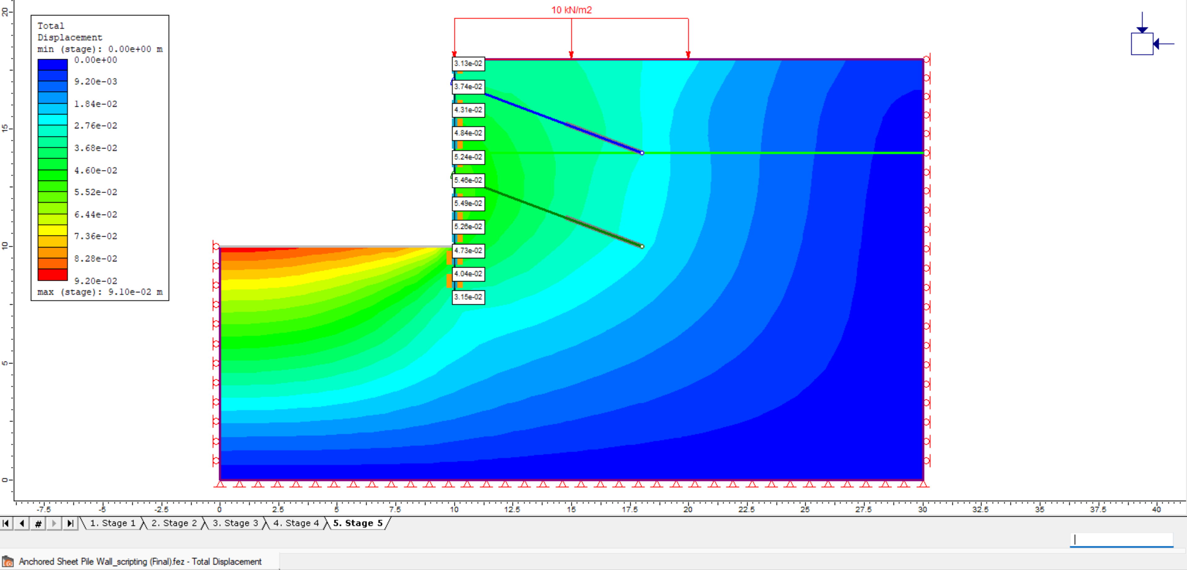
The total displacement results in RS2 Interpret will look as follows:
6.2 Liner Results
In Results Part II, we extract liner results at stage 5 including liner axial force, shear force, and bending moment. Results are outputted to CSV files and plotted.
Use .GetLinerResults() method to get all liner results at stage 5.
# Results Part II:
# Extract and plot axial force, shear force, and bending moment results at stage 5 for the liner

# Read liner axial force, shear force, and bending moment
liner_results = model_results.GetLinerResults(stages =[stage_number]) # output liner results on stage 5
Retrieve Liner 1 results.
stage_liner_results = liner_results[stage_number][0] #output the first liner results at stage 5Create a dictionary.
# Create a dictionary for the data frame and fill with first node data
liner_first_node = stage_liner_results.liner_element_results[0] # extrat first node data
liner_dict = {"Depth (m)":[18 - liner_first_node.start_y], # calculate depth from top of wall
 "Axial Force (kN)":[liner_first_node.axial_force1],
 "Shear Force (kN)":[liner_first_node.shear_force1],
 "Bending Moment (kNm)":[liner_first_node.moment1]}
The liner_element_results parameter from the LinerResults class returns a list of all liner elements within the liner. The first liner node data within Liner 1 has been added to the dictionary, including the Depth, Axial Force, Shear Force, and Bending Moment.
Since the element type for the model is 3-noded triangular, liner results are outputted at two nodes per liner element: start node and end node. If the model uses quadratic element type, liner result are outputted at three nodes per element. See the Liner Results Overview topic for more information.We now use a for loop to extract remaining liner nodes data to the dictionary in rows.
for liner_node in stage_liner_results.liner_element_results:
 # Add remaining data to the liner results dictionary
 liner_dict["Depth (m)"].append(18 - liner_node.end_y) # calculate depth from top of wall
 liner_dict["Axial Force (kN)"].append(liner_node.axial_force2)
 liner_dict["Shear Force (kN)"].append(liner_node.shear_force2)
 liner_dict["Bending Moment (kNm)"].append(liner_node.moment2)
Convert the dictionary to a DataFrame.
# Convert the dictionary to data frame
liner_results_df = pd.DataFrame(liner_dict)
Save the DataFrame as a CSV file: “liner results at stage 5.csv” to the results folder.
# Save the data frame to a csv
liner_results_df.to_csv(rf"{output_dir}\liner results at stage 5.csv", index=False)
6.3 Plot Liner Results
We will now plot the liner axial force, shear force, and bending moment diagrams.
A function is defined for plot formats using Matplotlib library methods.
# define a function to format plot
def format_plot():
 plt.gca().spines['bottom'].set_position(('data',0)) # move x-axis to y=0
 plt.gca().xaxis.set_label_position('top') # set x-axis label position to the top
 plt.gca().invert_yaxis() # invert y-axis
 plt.gca().spines['left'].set_position(('data',0)) # move y-axis to x=0
 plt.gca().spines['top'].set_visible(False) # hide the top spine
 plt.gca().spines['right'].set_visible(False) # hide the right spine
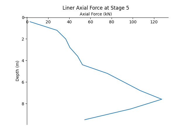
6.3.1 Liner Axial Force Diagram
- Plot the axial force values on x-axis and the depth along the liner on y-axis from the DataFrame.
Save the figure as “liner axial force at stage 5.png” to the results folder.
# Plot Liner Axial Force Diagram
plt.figure()
plt.plot(liner_results_df["Axial Force (kN)"], liner_results_df["Depth (m)"])
plt.xlabel("Axial Force (kN)")
plt.ylabel("Depth (m)")
plt.title("Liner Axial Force at Stage 5")
# format plot display
format_plot()
plt.gca().yaxis.set_label_position('left') # set y-axis label position to the left
# save plot
plt.savefig(rf"{output_dir}\liner axial force at stage 5.png")
The diagram will look as follows:
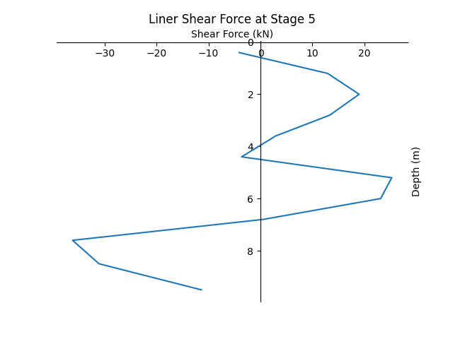
6.3.2 Liner Shear Force Diagram
- Plot the shear force values on x-axis and the depth along the liner on y-axis from the DataFrame.
- Save the figure as “liner shear force at stage 5.png” to the results folder.
# Plot Liner Shear Force Diagram
plt.figure()
plt.plot(liner_results_df["Shear Force (kN)"], liner_results_df["Depth (m)"])
plt.xlabel("Shear Force (kN)")
plt.ylabel("Depth (m)")
plt.title("Liner Shear Force at Stage 5")
# format plot display
format_plot()
plt.gca().yaxis.set_label_position('right')
# save plot
plt.savefig(rf"{output_dir}\liner shear force at stage 5.png")
The diagram will look as follows:
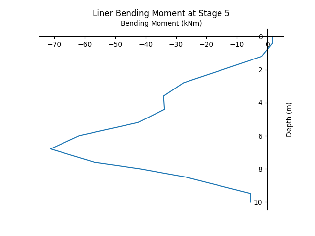
6.3.3 Liner Bending Moment Diagram
- Plot the bending moment values on x-axis and the depth along the liner on y-axis from the DataFrame.
- Save the figure as “liner bending moment at stage 5.png” to the results folder.
# Plot Liner Bending Moment
plt.figure()
plt.plot(liner_results_df["Bending Moment (kNm)"], liner_results_df["Depth (m)"])
plt.xlabel("Bending Moment (kNm)")
plt.ylabel("Depth (m)")
plt.title("Liner Bending Moment at Stage 5")
# format plot display
format_plot()
plt.gca().yaxis.set_label_position('right')
# save plot
plt.savefig(rf"{output_dir}\liner bending moment at stage 5.png")
The diagram will look as follows:
Display figures to the screen. You need to manually close the figure windows to finish the script.
plt.show()
# close the figure windows to finish the script
This concludes the Anchored Sheet Pile Wall Scripting tutorial.