Groundwater Flow in Cofferdam
1.0 Introduction
In this tutorial, finite element groundwater seepage analysis is used to determine the quantity of seepage entering a cofferdam. The model considers transient groundwater conditions and models the impermeable sheet pile boundary using a structural interface with an impermeable joint.
The example is based on problem 2.4 from Craig (1997).
This tutorial uses a model with pre-set project settings, geometry, material properties and meshing. The tutorial begins by defining groundwater conditions, then proceeds to the analysis of model results using RS2 Interpret.
2.0 Constructing the Model
- Select: File > Recent Folders > Tutorial Folder
- Open the initial file Groundwater Flow in Cofferdam (Initial).
2.1 Groundwater

The groundwater conditions consist of an initial steady-state stage, followed by an excavation stage, and finally, a pumping stage. The remaining stages following the pumping stage examine the variation of the groundwater conditions with time.
- Select the Groundwater workflow tab
- Select: Groundwater > Set Boundary Conditions

Stage 1:
- Select: Stage 1
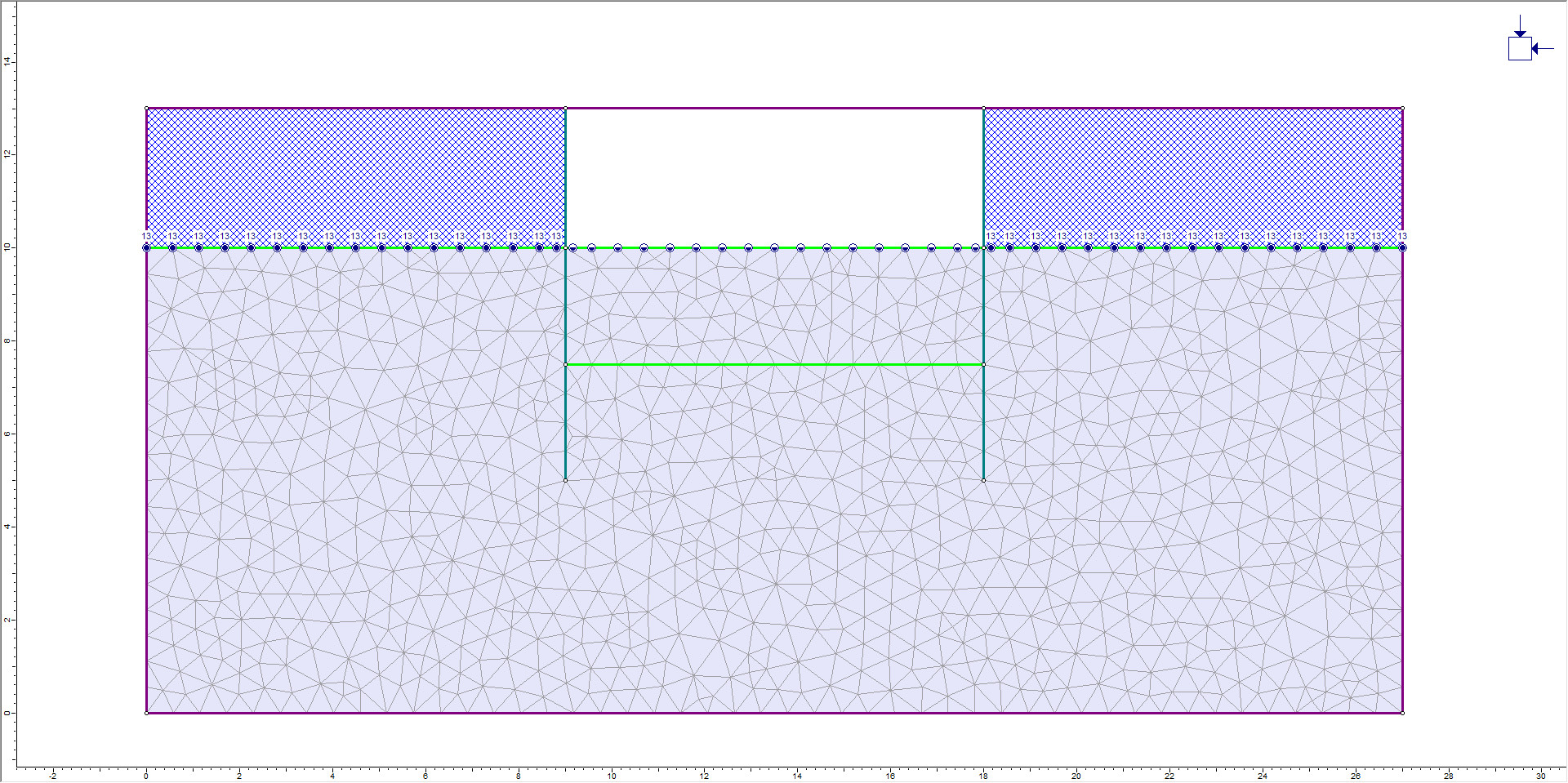
- Set Total Head as the boundary condition type. Enter 13m as the Total Head Value and choose “Boundary Segments” for the selection mode.
- Select the bottom of both the left and right excavated rectangles. Click Apply.
- Set Zero Pressure as the boundary condition type.
- Select the horizontal boundary between the two sheet pile walls. Click Apply.
The groundwater conditions will appear as follows:
Stage 2:
- Select: Stage 2
- Right-click on the zero pressure condition between the two sheet pile walls and select “Remove Boundary Condition.”
- Right-click on the lower material boundary between the sheet pile walls and select “Set Zero Pressure (P=0)”.
Stage 3:
- Select: Stage 3
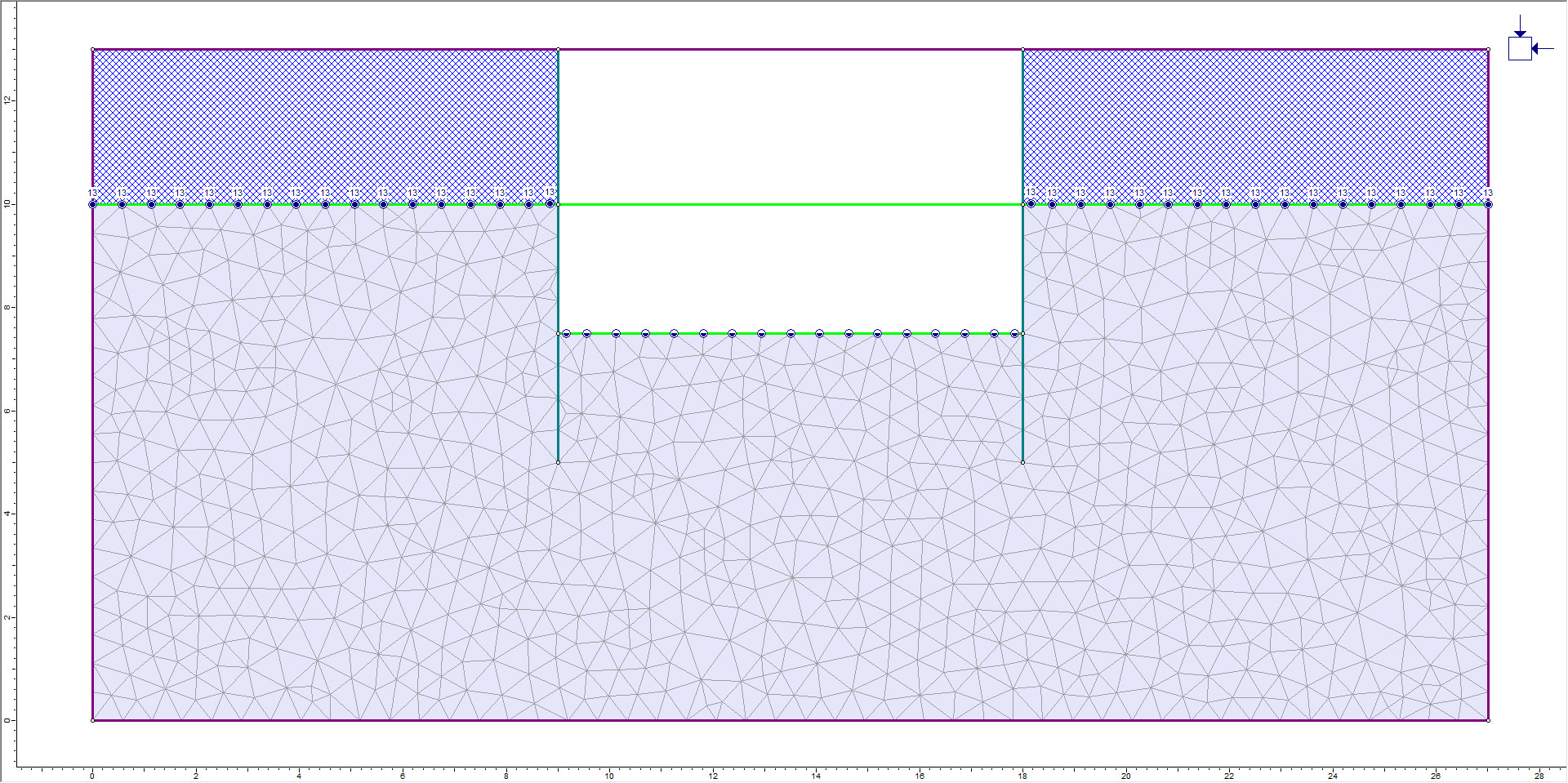
- Pumping conditions will be simulated in this stage. The elevation of the lower material boundary between the sheet pile walls is 7.5m. Therefore, a total head condition of 7m will be used to simulate pumping.
- Right-click on the boundary conditions on the lower material boundary between the sheet pile walls and select “Set Total Head.” Type 7m for the total head value and hit Enter.
The groundwater conditions will appear as follows:
Click through the first three stages to verify that the correct groundwater boundary conditions have been applied. The groundwater boundary conditions will not be changed for the remaining stages in the analysis (stages 4 to 11).
2.2 Discharge Sections
![]()
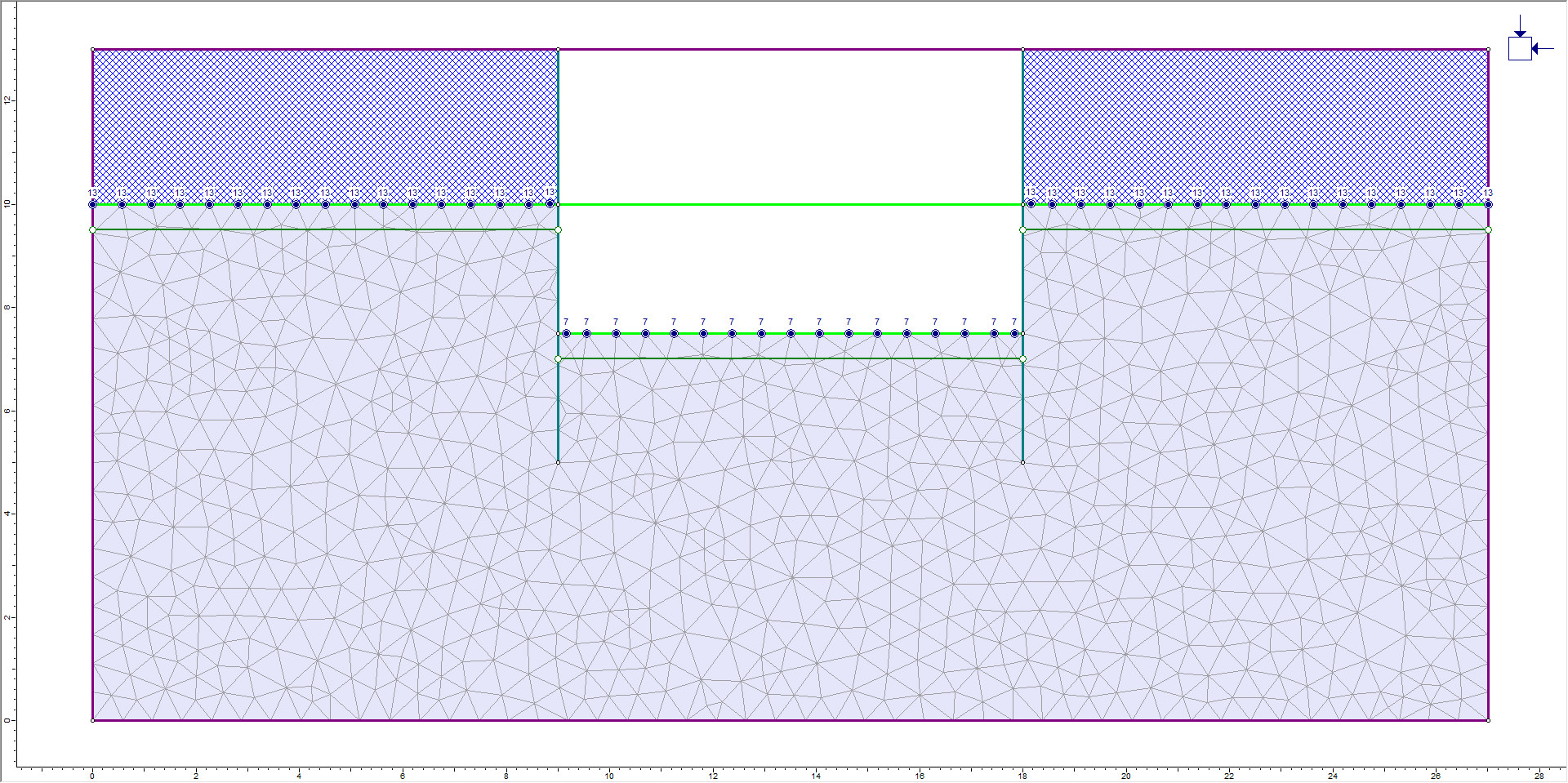
To calculate flow quantities, discharge sections must be added to the model. Three discharge sections will be used to gain an understanding of the groundwater flow in the model.
- Select: Groundwater > Add Discharge Section

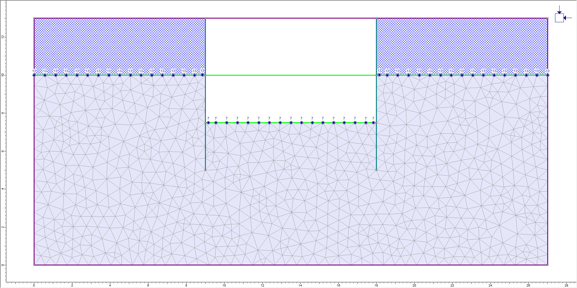
- Enter (0, 9.5) for the start of the section, then enter (9, 9.5). Hit Enter to end the discharge section.
- Add two more discharge sections with coordinates of (9, 7) to (18, 7), and (18, 9.5) to (27, 9.5).
Stage 3 of the model is shown below:
3.0 Compute
- Select: Analysis > Compute

4.0 Results and Discussion
- Select: Analysis > Interpret

The following screen shows the Pressure Head results for Stage 1 (Dam):
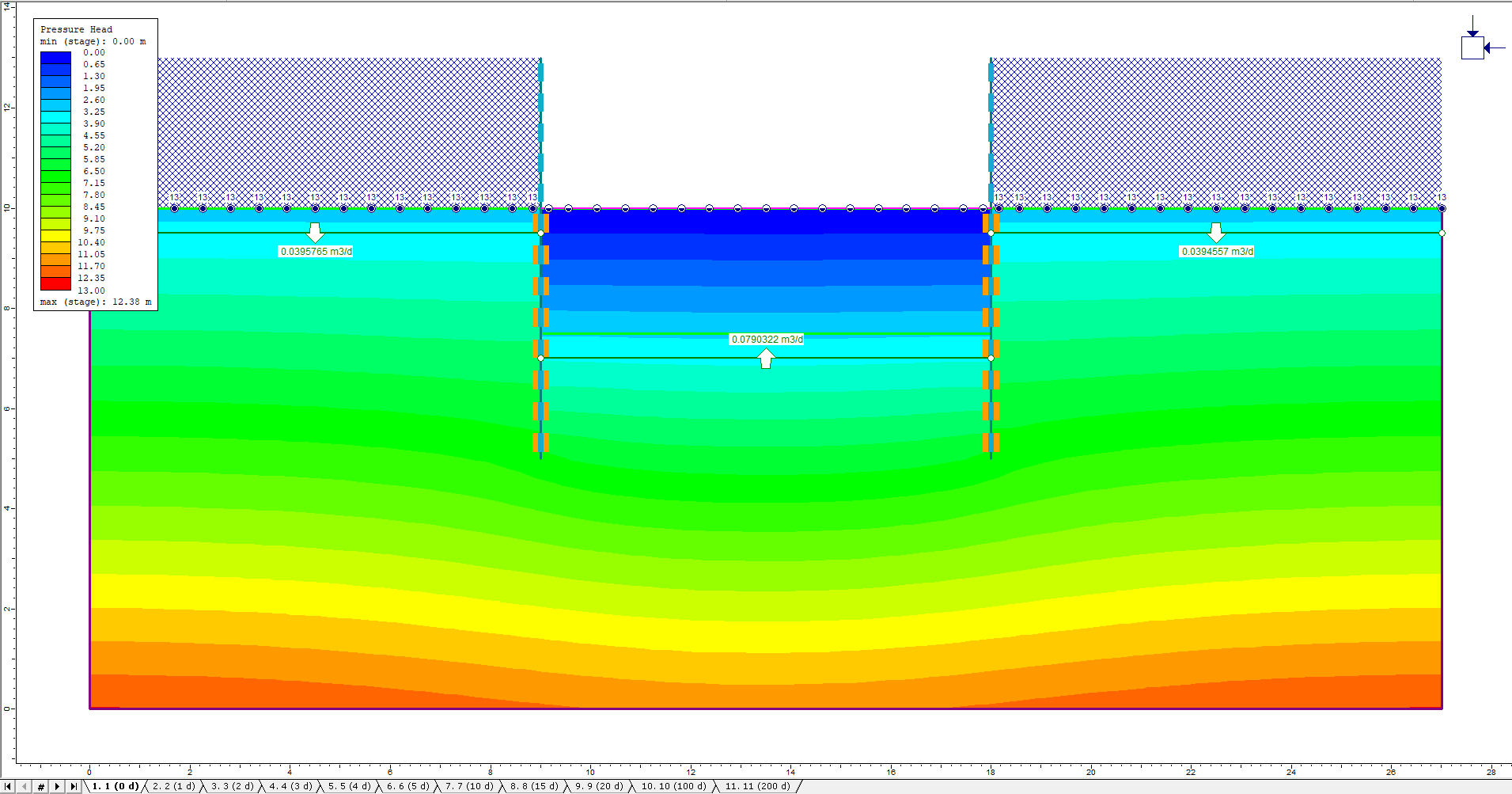
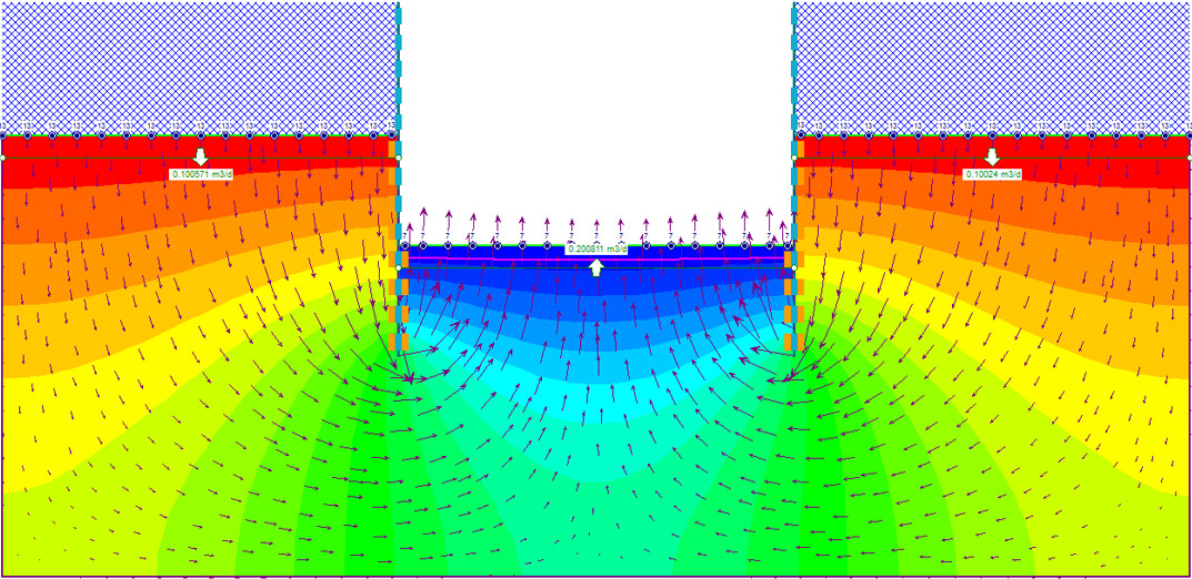
The volumetric flow rate and direction through each of the discharge sections are visible. As expected, the water is flowing down from the ponded water and up into the dam. The sum of the volumetric downwards flow is equal to the volumetric upwards flow between the sheet pilings. Note that in Stage 11 (200 days) the total downward flow rate on either side of the cofferdam (0.1 + 0.1) is equal to the total upward flow into the cofferdam (0.2) indicating that a steady-state condition has been reached.
 To see the magnitude and direction of flow throughout the model, plot the Flow Vectors.
The groundwater is flowing around the impermeable sheet pilings with high flow rates directly below the pilings. The image below shows the pressure head and flow vectors for Stage 4:
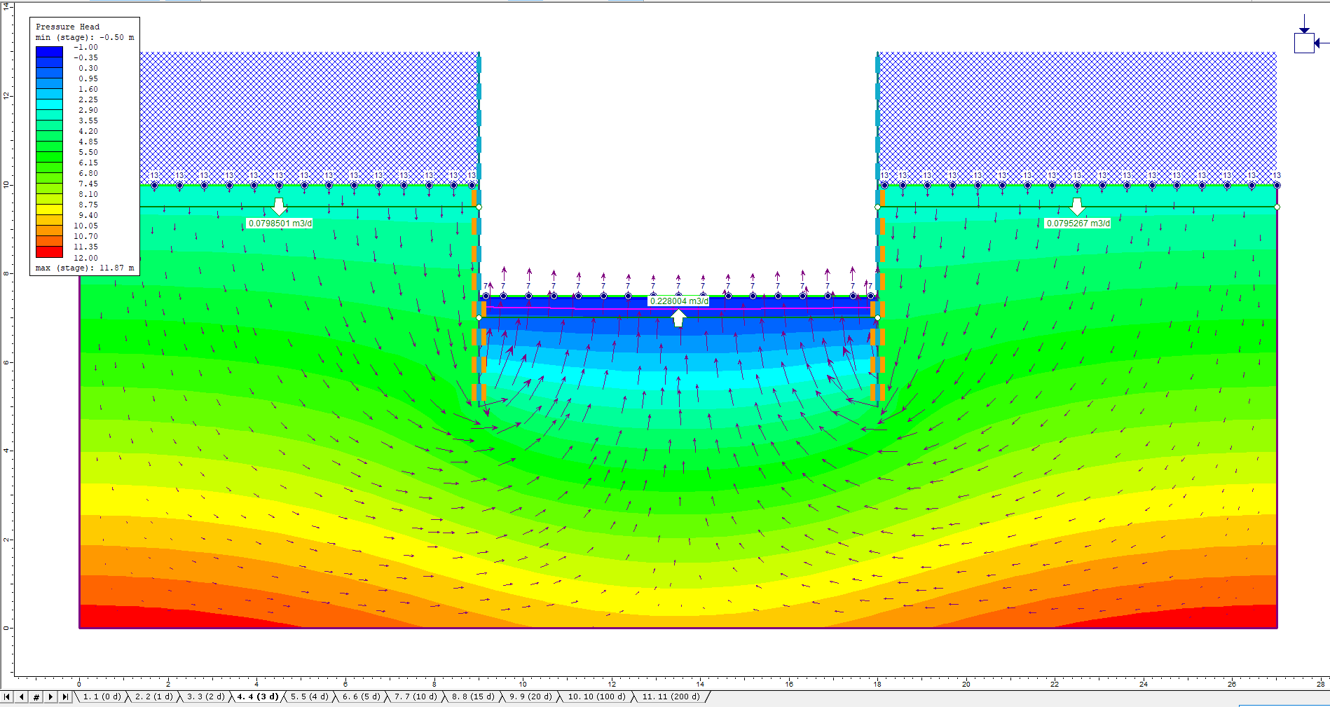
Because of the impermeable structural interface boundaries (impermeable joints), the water cannot flow through the cofferdam walls. Instead, the water flows down around the walls and up through the free surface at the bottom of the cofferdam.
Notice that in the early stages of the transient analysis, the discharge section flows are not balanced (i.e. total downward flow on either side does not equal the flow into the cofferdam).
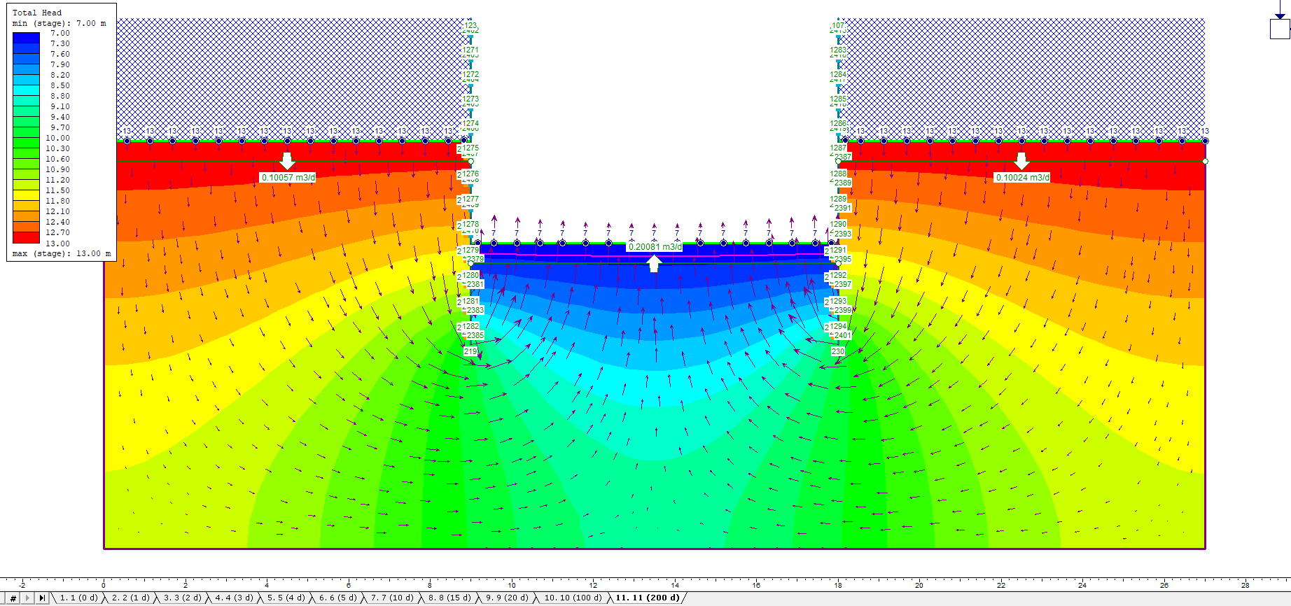
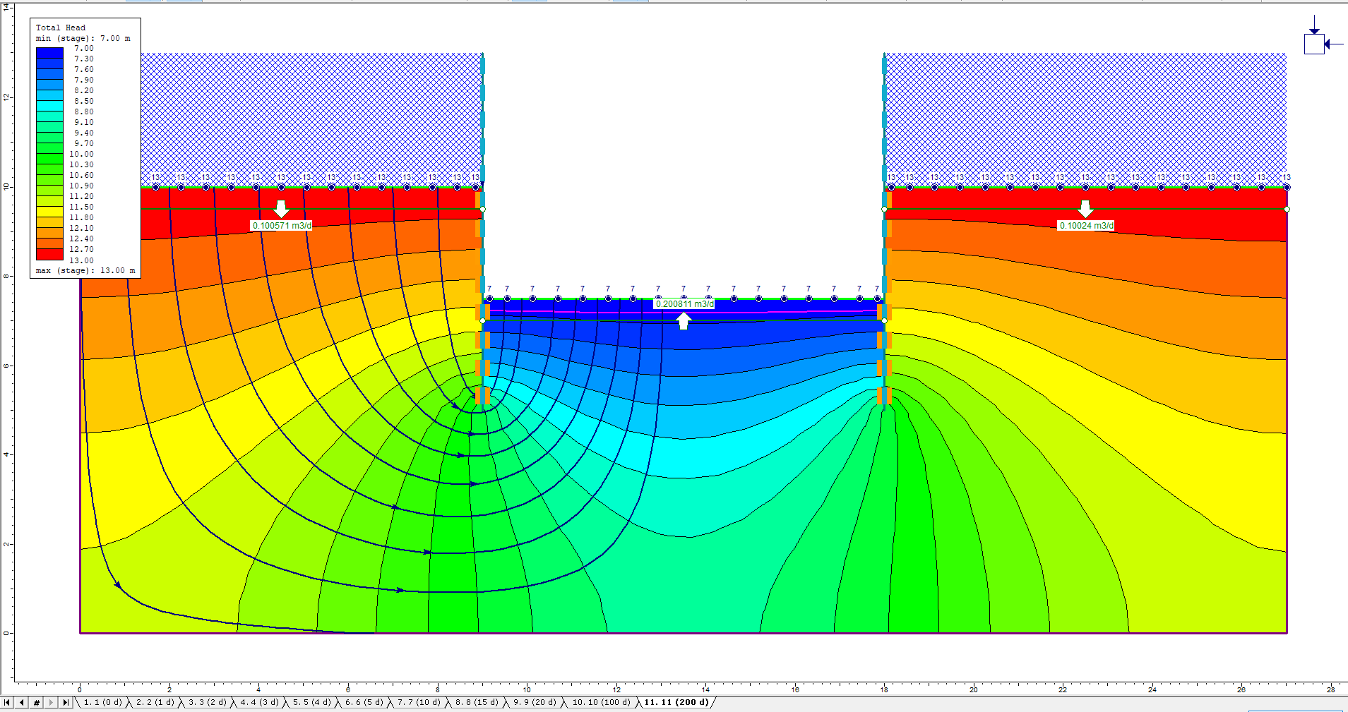
Now change the contours to Total Head and select the stages 1 to 11. Results for Stage 11 are shown below. Notice that the direction of the flow vectors is always in the direction of decreasing Total Head (i.e. flow vectors are perpendicular to the total head contours).
Notice the water table (pink line) is slightly below the bottom of the cofferdam since we defined a “pumping” condition by setting a Total Head boundary condition of 7 meters on the boundary which is at a 7.5-meter elevation.
A flow net can be constructed:
- Turn off the flow vectors by pressing the flow vector button again.
- Change the quantity being plotted from Pressure Head to Total Head using the drop-down menu on the toolbar.
- Right-click on the model and select Contour Options.
- Under Mode, select Filled (with lines), then Done. This will display the equipotential lines of the flownet.
To plot the flow lines:
- Select: Groundwater > Multiple Flow Lines.
- Select the top left corner of the soil as the first point. If the cursor does not snap to the node point, Select: View > Snap and ensure that all snap options are turned on.
- Now move horizontally until the cursor intersects the sheet piling and click to establish the second point.
- Press Enter.
- In the Flow Lines Options dialog:
- Under Flow Line Start Locations, select the first option and leave the default value (10 locations, evenly spaced along the entire polyline).
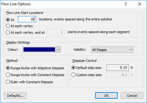
- Under Flow Line Start Locations, select the first option and leave the default value (10 locations, evenly spaced along the entire polyline).
- Click OK to close the dialog. 10 flow lines will be plotted as shown below.
- To complete the flownet, repeat these steps for the right side of the model.
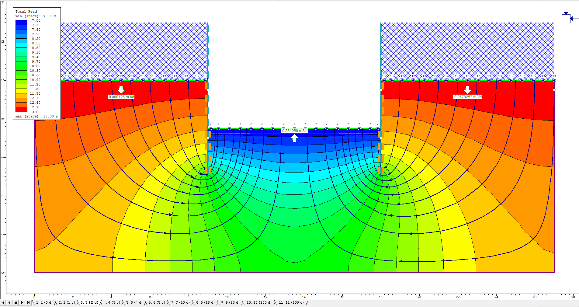
Now select the Stage 3 tab (Pump). For this stage, pumping was simulated by applying a total head lower than the elevation. The volumetric discharge at the bottom of the dam is higher than in Stage 2 and the water table has been lowered. The water table is shown as a pink line (water table line may be obscured by the green discharge line. To hide the discharge line, right-click on it and choose Hide This Discharge Section).
This concludes the Groundwater Flow in Cofferdam tutorial.
5.0 References
Craig, R.F., 1997. Soil Mechanics, Spon Press, London and New York, 485 pp.