Block Model

1.0 Introduction

Block Model is commonly used in mining industry to visualize the geological database and analyze complex soil and rock masses. A block model represents a rock/soil mass as a 3D gird of cubes (“block”), each assigned a material type and geotechnical properties. The underlying block database is stored as a point cloud, with each point containing information such as coordinates, material type, and properties.

Currently, among Rocscience products, block models are supported in Slide3, RS3, Slide2, and RS2, while direct database file import is available only in Slide3 and RS3.

In RS2, the block model feature allows you to import a Slide2 project where the block model is already defined.

In this tutorial, we will analyze an open pit project with block model in RS2. A Slide2 block model project has been prepared beforehand, and we will start by bringing it into RS2. Note that:

• The Slide2 block model project is created by exporting a 2D section from a Slide3 block model project, where the block database file was first imported. The complete workflow is: block database file > Slide3 > Slide2 > RS2.
• The model used in this tutorial is the same as in the RS3 Block Model Tutorial.
• The finished product can be found under File > Recent > Tutorial Folders > Slope Stability folder path, in the Block Model (final).fez file.

2.0 Constructing the Model

2.1 Import Slide2 File

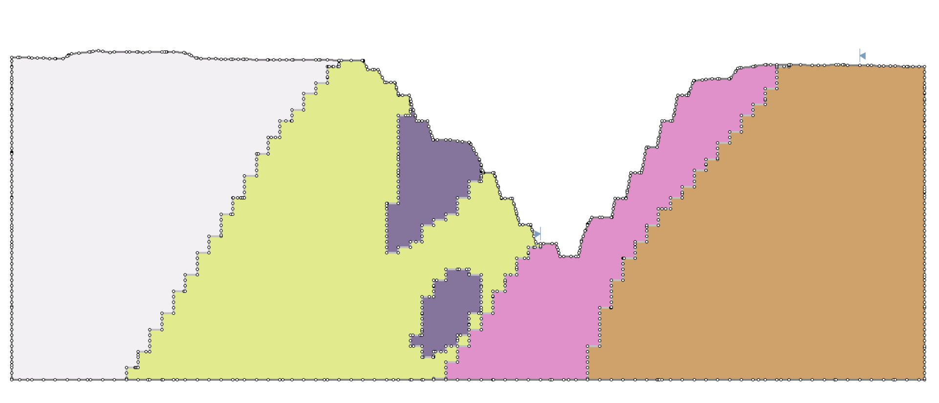
Let’s start by importing the Slide2 block model project. The project has block model data projected to the geometry, and as a result, the strength parameters for each material vary throughout the domain. It looks as follows in Slide2:

1. Open the RS2 Modeler program.
2. Select File > Import > Import Slide..
3. In the Open dialog, select the Slide2 file: Block Model (initial).slmd from the folder path:
   C:\Users\Public\Documents\Rocscience\RS2 Examples\Tutorials\Slope Stability
4. In the prompted Slide Import Options dialog, uncheck the Automatically Generate Boundary Conditions and Automatically Generate Mesh option. The dialog should look as follows:
   
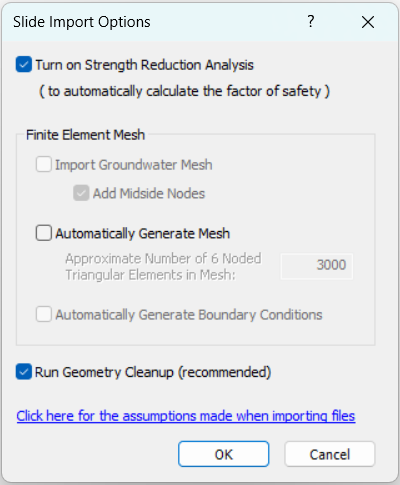
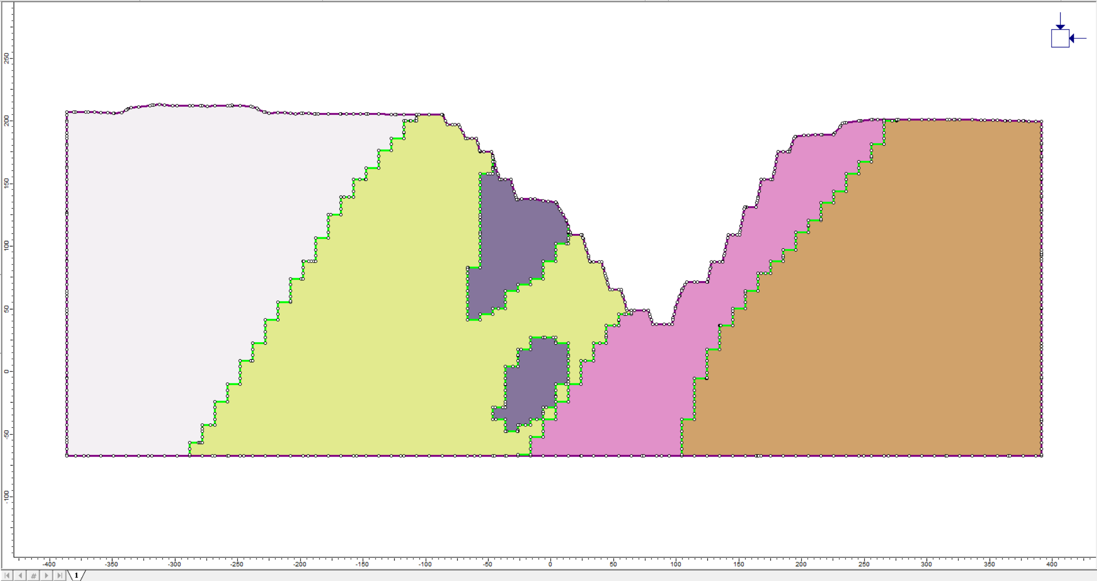
5. Click OK to proceed. Now the Slide2 file is successfully imported into RS2, with Geometry Cleanup completed and SSR Analysis turned on. The model should look as follows:
   

2.2 Project Settings

1. Select: Analysis > Project Settings
2. Select the Strength Reduction tab, ensure the Determine Strength Reduction Factor option is checked. The dialog should look as follows:
   
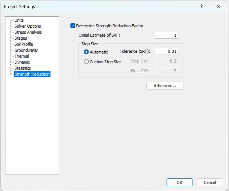
3. Leave all parameters as the default settings, click Cancel to exit.

2.3 Material Properties

Now we look at the block model material properties.

1. Select the Materials & Staging workflow tab.
2. Select: Properties > Define Material Properties
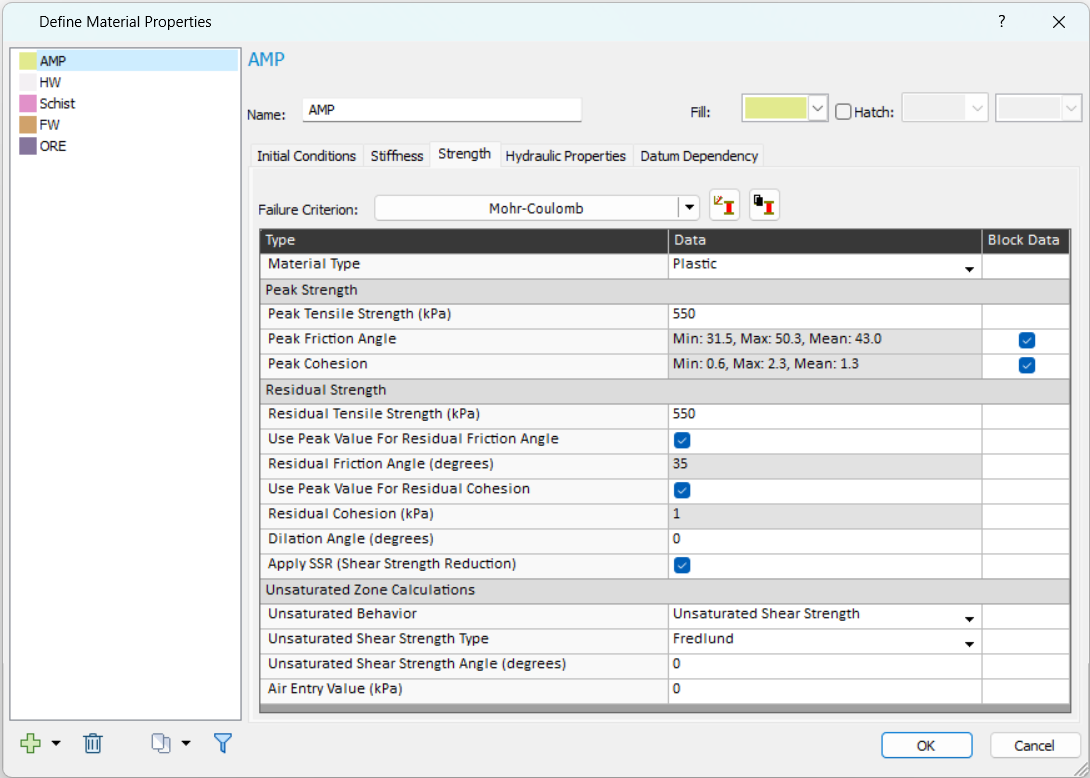
3. Select material AMP (Amphibolite) from the list in the left of the dialog, and go to the Strength tab.
   
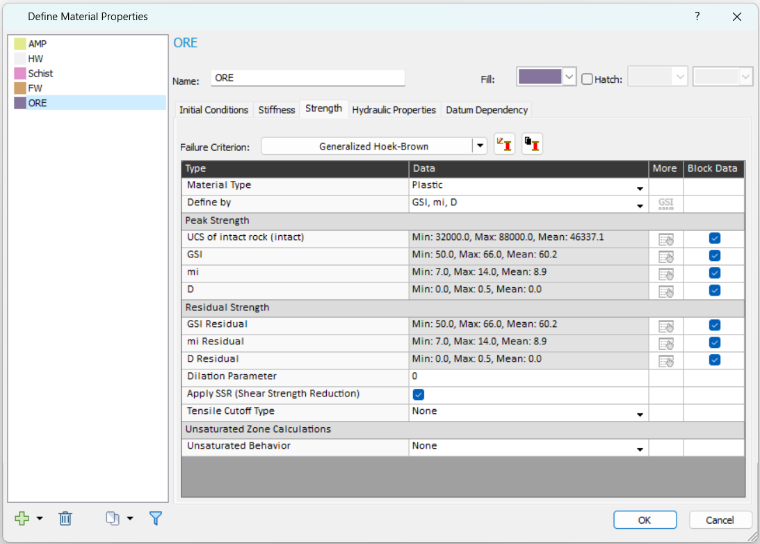
   You will see an extra Block Data column, which appears only for models that contain block data.
   The Block Data checkbox is available only for parameters with block-level data. When selected, the parameter will use the block data; the Data field will then be disabled, and the Min, Max, and Mean values of the block data across the selected material will be displayed. If you prefer not to use block data, you can clear the checkbox and input a value manually.
   
4. Select the checkboxes for Use Peak Value for Residual Friction Angle and Use Peak Value for Residual Cohesion. The block data for peak friction angle and cohesion are now applied as the residual values. The dialog should look as follows:
   
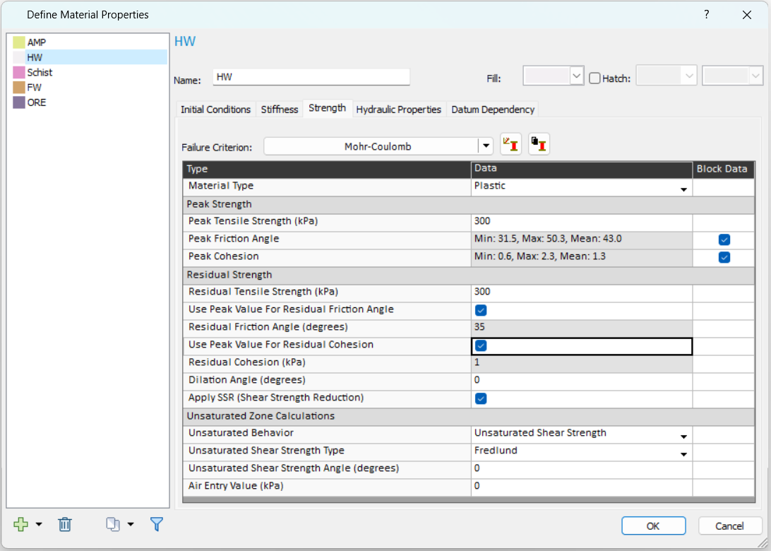
5. Select material HW (Hanging Wall) from the list.
6. Under the Strength tab, select the checkboxes for Use Peak Value for Residual Friction Angle and Use Peak Value for Residual Cohesion, as follows:
   
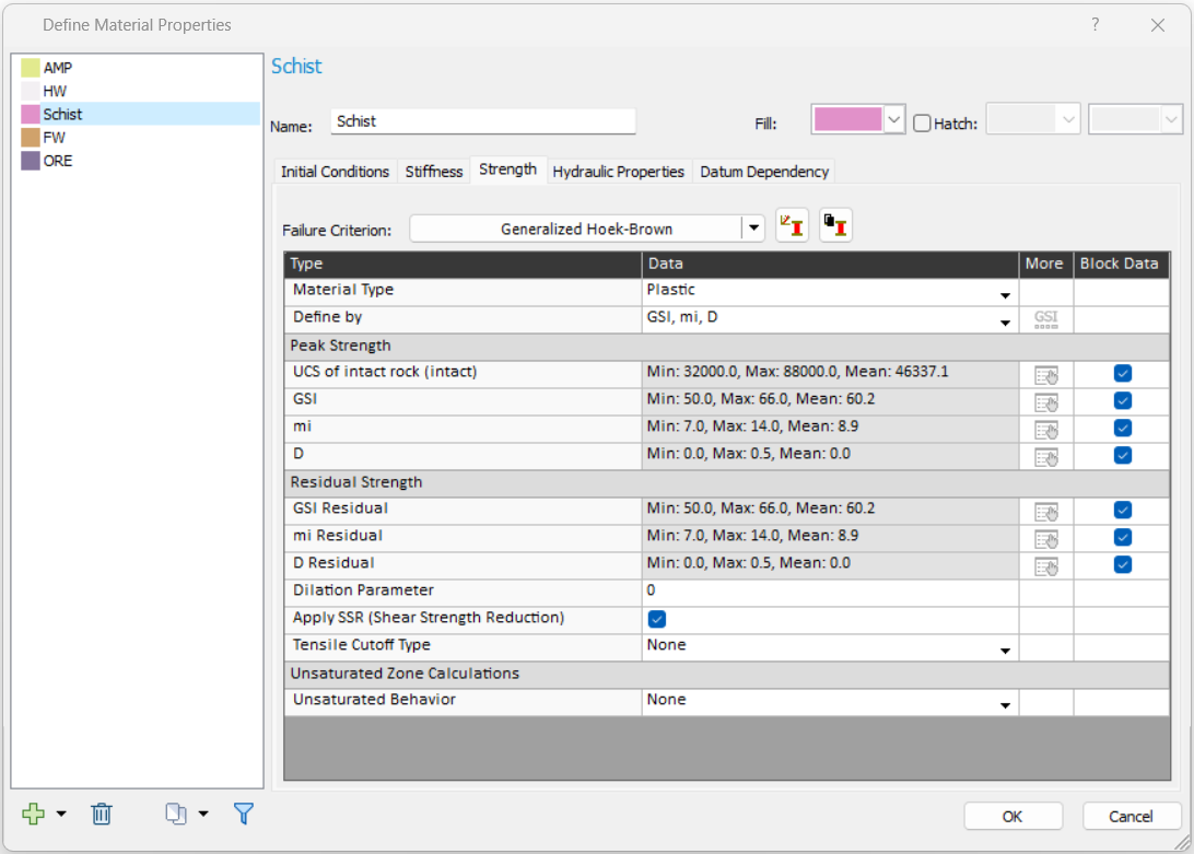
7. Select material Schist from the list.
8. Under the Strength tab, note that for Generalized Hoek-Brown model, block data are automatically applied to residual parameters. Leave default settings as shown:
   
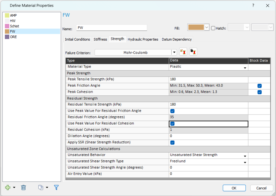
9. Select material FW (Foot Wall) from the list.
10. Under the Strength tab, select the checkboxes for Use Peak Value for Residual Friction Angle and Use Peak Value for Residual Cohesion, as follows:
    
11. Select material ORE from the list. Under the Strength tab, leave default settings as shown:
    
12. Click OK to apply and exist the dialog. Material properties are now defined.

2.4 Mesh

1. Select the Mesh workflow tab.
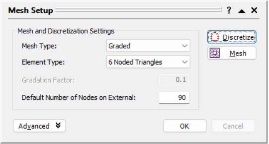
2. Select: Mesh > Mesh Setup
3. We will use the default mesh settings as shown below. Select Discretize and Mesh.
   
4. After mesh has been generated, click OK to exit the dialog.

2.5 Check Mesh Quality

Now, let’s check the mesh quality of the geometry to detect and prevent potential issues in the analysis (i.e., non-convergence caused by numerical issues).

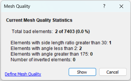
1. Select: Mesh > Mesh Quality > Show Mesh Quality
2. In the Mesh Quality dialog, as shown below, two elements with poor mesh quality are detected.
   
3. Click Show. The targeted elements will be highlighted in the model, as shown below.
   
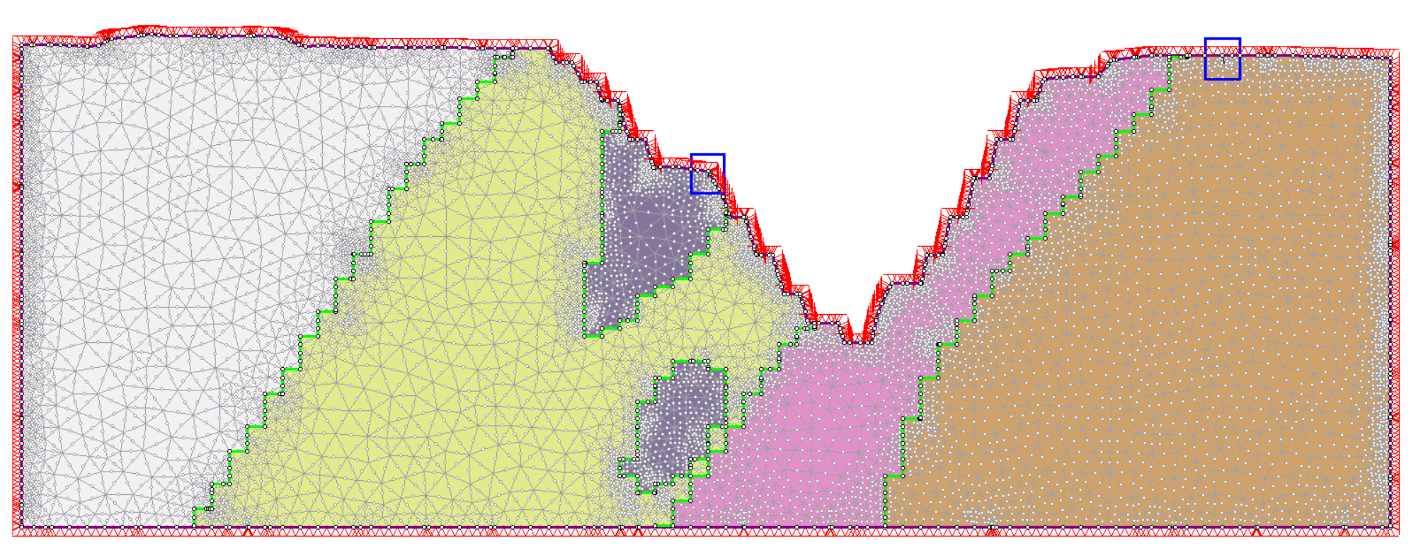
   Let’s clean them up.
4. Select the Geometry workflow tab at the top.
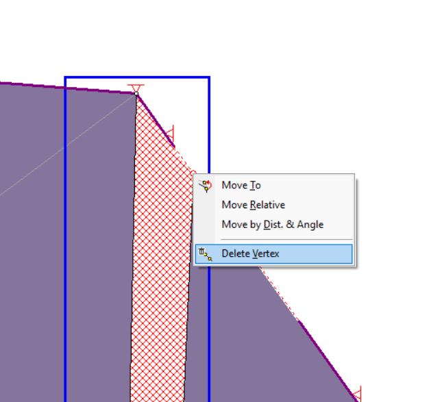
5. Zoom in to the left highlight first. As shown below, it can be seen that the two vertices for this triangular mesh element are too close. Right-click on the right vertex and select Delete Vertex from the list.
   
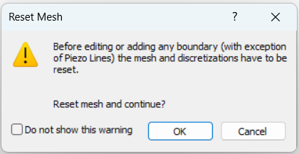
6. In the prompted Reset Mesh warning dialog, select OK.
   
   The vertex will be removed along with mesh. Let’s clean up the other poor quality mesh element.
   
   
7. Select Mesh > Discretize and Mesh
8. Select Mesh > Mesh Quality > Show Mesh Quality , and click Show.
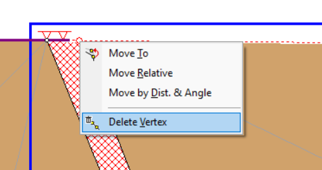
9. Zoom in to the highlighted area in the model. As shown below, similar to the first one, the two vertices are too close.
10. Right-click on the right vertex, select Delete Vertex, and select OK to the prompt warning.
    
    Let’s check again.
    
    
11. Select Mesh > Discretize and Mesh
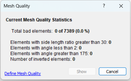
12. Select Mesh > Mesh Quality > Show Mesh Quality . As shown below, poor meshes have been cleaned. Click Cancel to exit.
    

2.6 Restraints

Now we define the restraints.

1. Select the Restraints workflow tab.
2. Select Displacements > Free
3. In the Set Restraints/Displacements dialog, set Selection mode = Boundary Nodes, as follows.
   
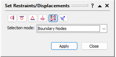
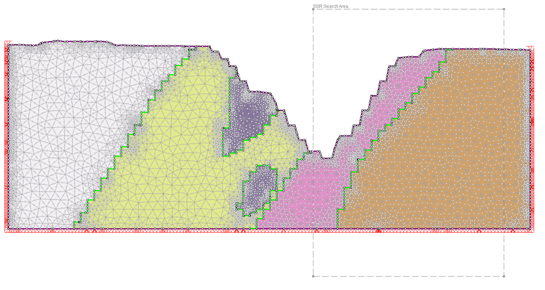
4. In the viewport, use the selection tool to drag to include the top boundaries, except for the two end vertices at the top corners. Click Apply in the dialog. Your model should look as follows.
   
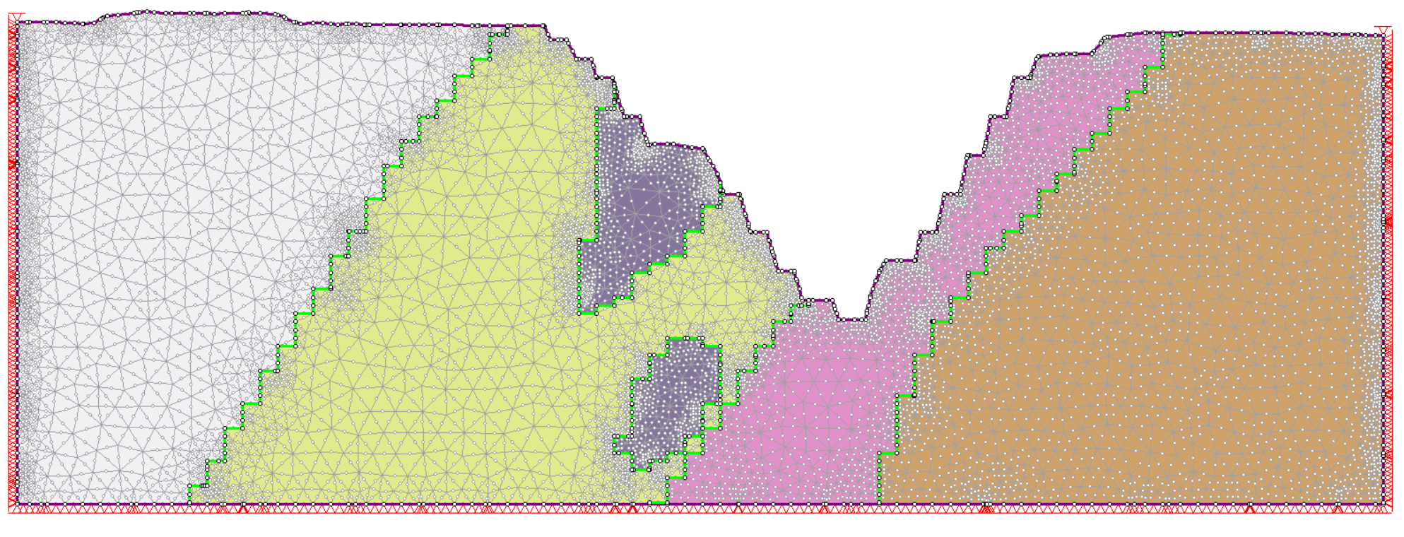
5. Click Close to exit the dialog.

2.7 SSR Search Area

To focus slope stability on critical region, we will define a SSR Search Area to match with the defined limited search area in Slide2.

1. Select: Analysis > SSR Search Area > Define SSR Search Area (window)
2. Use the crosshair tool, click and drag to define a rectangle at the position shown below as the SSR search area. Alternative, you can input two point coordinates (68, 260) and (352, -130).
   

3.0 Compute

1. Select: File > Save As to save the model as Block Model (final).fez
2. Select: Analysis > Compute

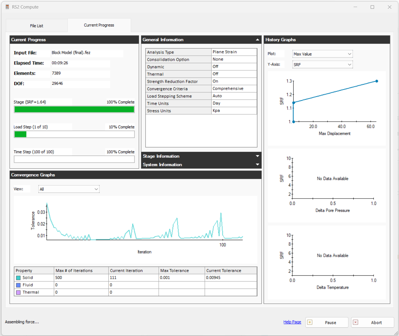
During computation, in the RS2 Compute UI under the Current Progress tab, you can monitor the updates through the convergence graphs and various history graphs.

4.0 Results

1. Select: Analysis > Interpret
   The critical strength reduction factor (SRF) appears at the top of the screen. By default, the Maximum Shear Strain result is displayed. Use the tabs along the bottom of the screen to view results for different SRF values.

4.1 SRF

1. Switch to tab: SRF:1.23 (r)
   As seen below, the surface of failure falls within the SSR search area.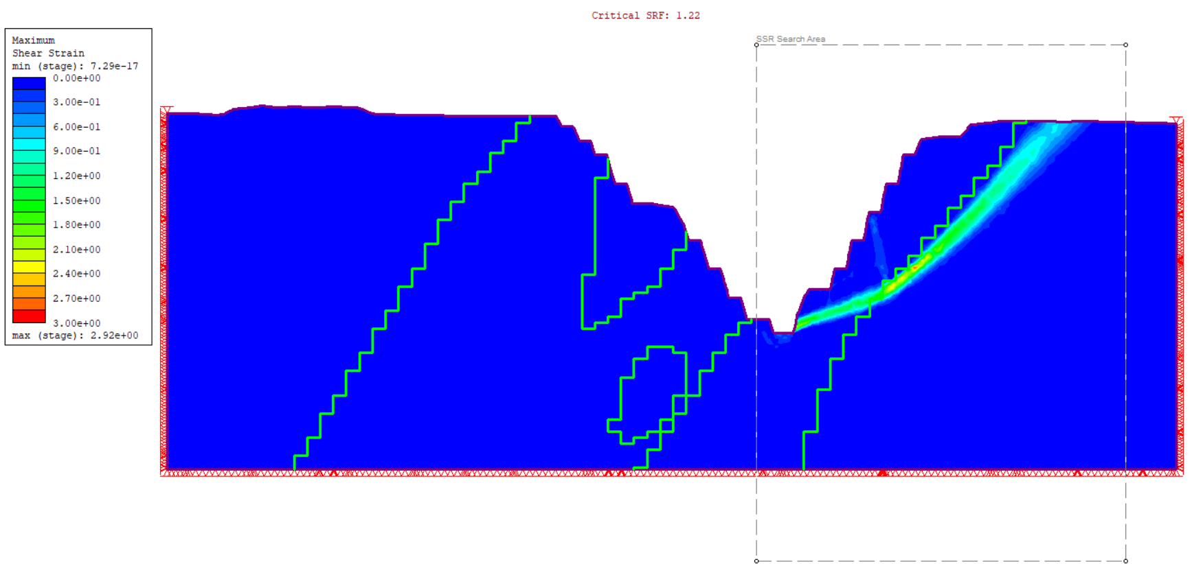
   
   Below shows results from Slide2 Interpret. Compare RS2 results with Slide2, where the factor of safety is 1.263 with Spencer method and 1.254 with GLE/Morgenstern-Price method, they are close matches with the critical SRF of 1.22 in RS2.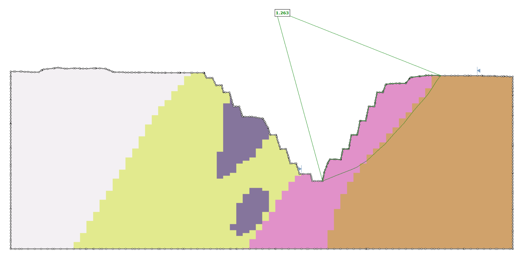
   

4.2 Total Displacement

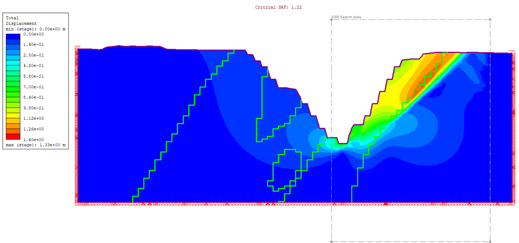
1. Set result type to Solid Displacement > Total Displacement, and switch tab to SRF:1.22 (r)
2. As shown below, the largest displacement happens along the failure slope of 1.33m.
   
   You can explore to view other result contours in RS2 Interpret. This concludes the RS2 block model tutorial.