Application of Joint Networks
1.0 Introduction
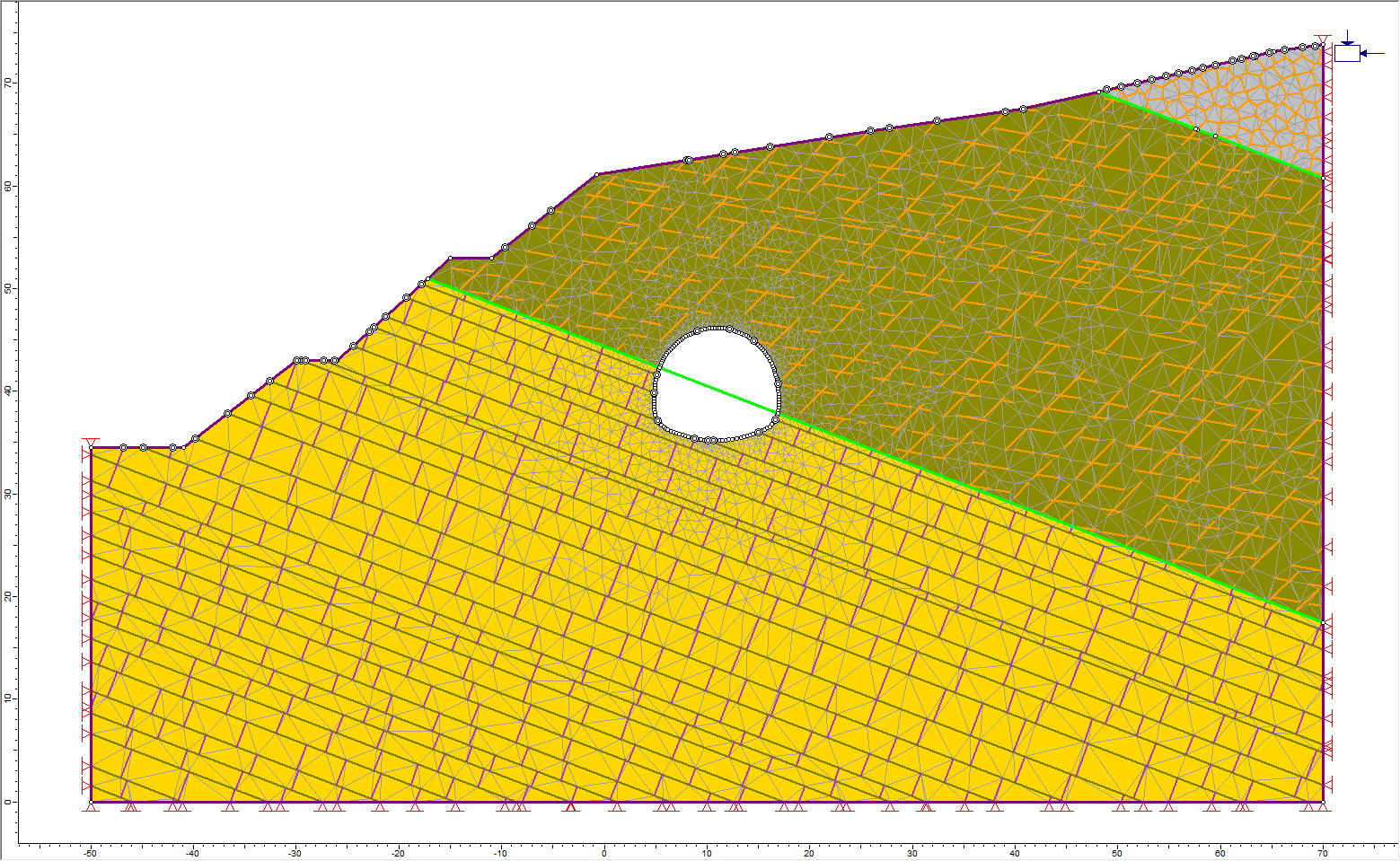
This tutorial will demonstrate how to specify joint networks or discrete fracture networks (DFN) in RS2 using the automatic joint network generator. It will also demonstrate techniques for analyzing the effects of the joints on model results. The model involves the stability analysis of a transportation tunnel near a slope in blocky rock. There are three different zones of blocky rock in the model.
2.0 Constructing the Model
- Select: File > Recent Folders > Tutorial Folder > Jointed Rock
- Open Application of Joint Networks (Initial)
2.1 Adding a Voroni Joint Network Zone 1

Let’s apply a joint network to the zone at the upper right corner of the model.
- Select: Boundaries > Joint Networks > Add Joint Network

- Notice that the mouse cursor immediately changes shape. Click the left mouse button at any location within Zone I (upper right corner). A hatched pattern appears in the selected zone. Hit Enter or right-click and select Done to complete zone selection. The Add Joint Network dialog pops up:
Input data fields are grouped under headings. Labels (descriptions) of the input fields are shown on the left cells while the corresponding actual input fields are on the right.
Automatic Preview of Joint Networks
The third check box in the lower section of the joint network dialog is labeled “Update Preview”.
- A preview of the currently active joint network is displayed on the RS2 model being developed, as soon as the joint network dialog appears.
- When the “Update Preview" check box is on (the default status), a joint network is immediately redrawn the moment any change is made to a parameter in the dialog. When it is off, the preview remains but will not be updated until the dialog is closed. Leave the Update Preview check box on.
The network is shown in a rectangular window slightly larger than the selected zone. In addition to allowing you to see the geometry of the joint network you are specifying; the preview feature allows you to zoom into any part of a model for a closer look without leaving the joint network dialog.
- Zoom into an area of the model around Zone I to take a closer look at the currently displayed joint network. Press F2 when done to reset the view to the model extents.
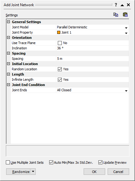
Specifying Input for Voronoi Joint Network
Under the General Settings heading in the dialog, click on the Joint Model input field (the cell on the right with the descriptor Parallel Deterministic). In the resulting dropdown menu:
- Select the Voronoi model. Notice that the joint network displayed on the model immediately changes (depending on the speed of your computer the preview may not be as quick.)
- Change the Density (number of Voronoi cells per unit area) to 0.4.
- Once the network of Voronoi cells is displayed, click on the Regularity input field and change the option from Irregular to Medium Regular.
Changing Joint End Conditions
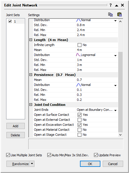
By default, the ends of all joints in a network are assumed to be closed, i.e. no relative movement (joint sliding or opening) can occur at a joint end. Options exist in the joint network dialog for removing this constraint. In this example, specify that joint ends be open at the ground surface and at intersections with the excavation (tunnel).
- Click on the input data cell (cell with the default end condition setting of All Closed).
- Select "Open at Boundary Contacts" from the dropdown list. Once this option is selected, five new rows of data appear. Each row describes end conditions for joints that intersect a type of boundary (there are five types of boundaries in RS2.)
- In a model, the first time the Open at Boundary Contact option is selected, joint ends are specified as open at the ground surface and at excavation boundaries. Accept these defaults. The dialog should appear as below. Select the OK button to close the dialog.
This completes the specification of a joint network for Zone I.
2.2 Adding a Network Comprising Two Joint Sets to Zone II
![]()
Let’s apply a joint network to Zone II of the model. This time the network will contain two sets of parallel joints.
- Select: Boundaries > Joint Networks > Add Joint Network
- Click the left mouse button anywhere within Zone II and hit Enter to complete selection. The joint network dialog pops up.
There are three checkboxes towards the bottom of the joint networks dialog.
- The first check box, Use Multiple Joint Sets, allows the specification of a network with more than one joint set.
- The second check box, Auto Min/Max 3x Std. Dev., is on by default. It automatically calculates lower and upper bounds (relative minimum and relative maximum values) for the values generated from a statistical distribution based on the specified standard deviation.
The Auto Min/Max 3x Std. Dev. option calculates both relative minimum and relative maximum as three times the standard deviation. However, there are exceptions. If a relative minimum or maximum calculated this way will result in an invalid bounding value (for example, if it leads to negative spacing), the minimum or maximum will be assigned a lower value that maintains a valid bound.
- Select the Use Multiple Joint Sets check box.
A new panel appears on the left side of the dialog as soon as the option is turned on. The panel shows an automatically selected joint set – Joint Set 1.
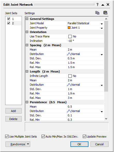
Setting the Parameters for Joint Set 1
For Joint Set 1:
- Change the joint model to Parallel Statistical.
- Leave the joint property field as Joint 1.
- Under the Orientation section of the dialog, leave the Use Trace Plane option as the default of "No". Enter an inclination angle of 45.
Next, specify a distribution for the spacing of the parallel joints in Set 1:
- Enter a mean spacing of 3 m.
- Leave the choice of distribution as Normal.
- Set the standard deviation to 0.8.
Because the Auto Min/Max 3x Std. Dev. option is on, the relative minimum and relative maximum values for the distribution are automatically calculated. Both relative minimum and relative maximum are automatically set to a value of 2.4 (3 x 0.8).
Input parameters for the length of joints:
- Change the Infinite Length option from Yes to No. Once you do this several new input data fields appear for entering parameters for the distribution of joint lengths. Specify the following values:
- Mean = 4 m
- Distribution = Lognormal
- Standard deviation = 1 m.
- The relative minimum and maximum values are again set automatically.
- For persistence, specify the following distribution parameters:
- Mean = 0.7
- Distribution = Normal
- Standard deviation = 0.1.
- The relative minimum is automatically set to 0.3 (3 x 0.1). The relative maximum is however set to only 0.2. This is because a persistence of 1 is not allowed.
- Change the Joint End Condition to Open at Boundary Contacts as we did for the previous network. The dialog should now look as follows:
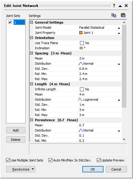
This completes the definition of Joint Set 1.
Setting the Parameters for Joint Set 2
When the Use Multiple Joint Sets option is selected, Add and Delete buttons appear beneath the left panel with joint sets information.
- Click on the Add button. A second joint set labeled Joint Set 2 shows up on the left panel just below Joint Set 1. It is highlighted, indicating that Joint Set 2 is active, and its parameters can be specified or altered.
Notice that there are checkmarks beside the joint set labels.
A checkmark indicates that a joint set is drawn (or applied) in the selected material zone. If deselected, although the data (parameters) for the joint set remain, joints from the set are not applied to the material zone. Leave the checkmarks as is.
- For Joint Set 2, input the parameters shown in the table below. Leave all other parameters as the defaults provided in the dialog.
Parameter |
Value |
| General Settings Joint Models Joint Property |
|
Orientation |
|
Spacing |
|
Length |
|
Persistence |
|
Joint End Condition |
Open at Boundary Contacts |
Now the dialog for Joint Set 2 should look as follows:
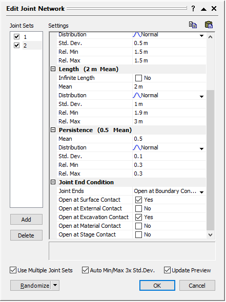
- Click on the OK button to complete the definition of the joint network for Zone II.
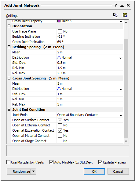
2.3 Adding a Cross-Jointed Network to Zone III
![]()
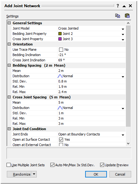
Let’s apply a fracture network consisting of bedding planes with cross joints to Zone III.
- Select: Boundaries > Joint Networks > Add Joint Network
- Click the left mouse button anywhere within Zone III and hit enter to complete selection.
- In the joint network dialog:
- Specify the parameters indicated in the table below for the cross-jointed network.
- Leave any other parameters not specified as the defaults provided in the dialog.
- Click on the OK button to close the joint network dialog and apply the joint network to Zone III.
| Parameter | Value |
General Settings |
|
Orientation |
|
Bedding Spacing |
|
Cross Joint Spacing |
|
Joint End Conditions |
|
The dialog should look as follows:
This completes the specification of joint networks for the model.
2.4 Field Stress

- Select: Loading > Field Stress

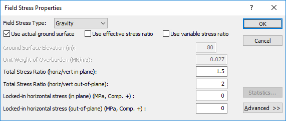
- Enter the parameters indicated in the field stress dialog above. Select OK. Notice that in this tutorial, horizontal stresses are assumed to be larger than the vertical stresses.
2.5 Mesh
![]()
- Select: Mesh > Discretize and Mesh

- If a “Joint Networks Warning” dialog appears, click Clean geometry. This process is recommended when using joint networks to ensure good mesh quality.
- In the Geometry Cleanup dialog, accept the default values and click OK.
- Select Yes to the discretization and mesh prompt which follows.
The model should appear as shown below:
2.6 Boundary Conditions
![]()
The slope (ground) surface is not free; it has pinned (fixed, zero displacement) boundary conditions. This occurs because by default all nodes on the external boundary are pinned.
To remove these conditions:
- Select: Displacements > Free

- Use the mouse to select all the line segments that define the ground surface.
- When finished, right-click on the mouse and select Done Selection. The triangular pin symbols should now be gone from the slope surface.
It may be necessary to re-apply the pinned boundary conditions to the uppermost nodes of the left and right external boundaries of the model. To do so:
- Select: Displacements > Restrain X,Y

- Right-click the mouse. Select Pick by Boundary Nodes from the resulting popup menu. This will change the mode of application of boundary conditions from segments to nodes.
- Select the topmost vertex of the left external boundary with coordinates (-50, 34.5) and the corresponding vertex on the right boundary with coordinates (70, 73.761)
- Right-click and select Done Selection. Triangular pin symbols now appear at these vertices.

3.0 Compute
- Select: File > Save As

- Select: Analysis > Compute

Since the model uses plastic materials and joints, the analysis may take some time.
4.0 Results and Discussion: With Support
- Select: Analysis > Interpret

4.1 Contours of Major Principal Stress – Sigma 1
Contours of major principal stress, Sigma 1, will be displayed.
The following contours should be visible:
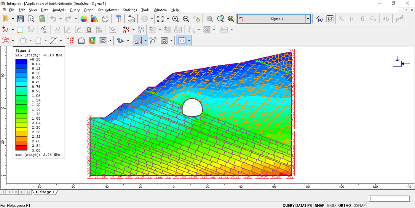
The effects of the joints on the Sigma 1 contours are visible; the contours are jagged and not as smooth as those for models without joints.
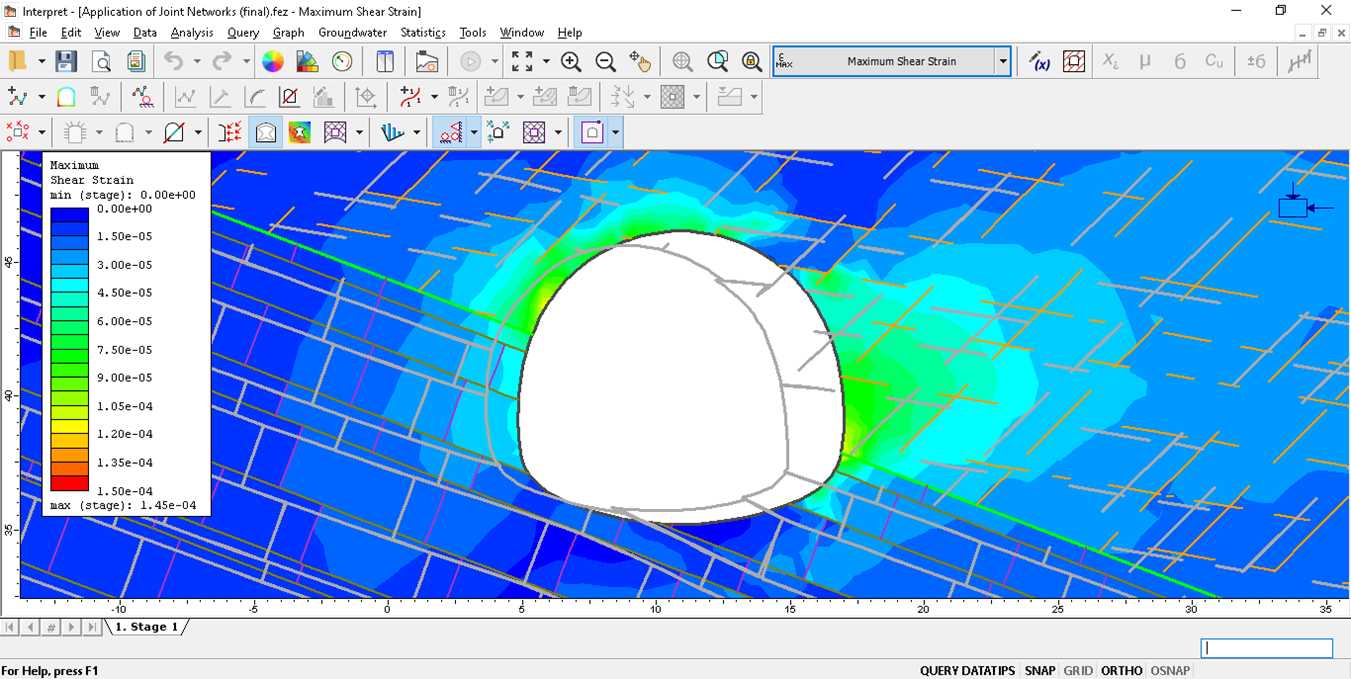
4.2 Contours of Maximum Shear Strain
- Select Maximum Shear Strain from the drop-down menu in the toolbar.
The contours reveal that very little shear strain occurs in the intact rock materials (most of the model is coloured in blue). Most of the shear displacements must be occurring along the joints.
Zoom in on the excavation to examine the distribution of shear straining in that region.
- Select: View > Zoom > Zoom Excavation

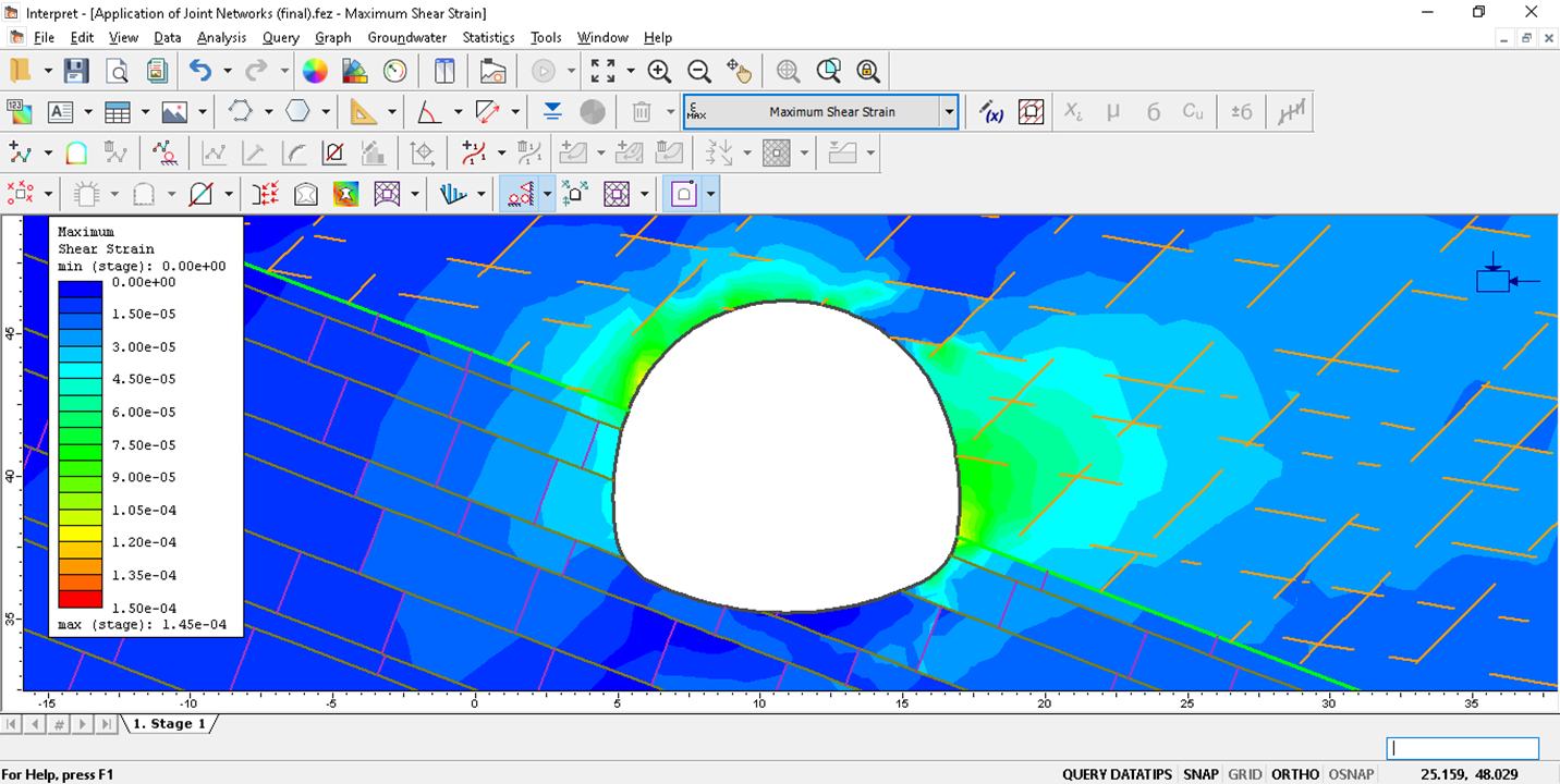
Concentrations of shear strain occur at some joint ends and joint intersections with the tunnel.
4.3 Deformed Boundary
RS2 Interpret can display an exaggerated view of the deformed shapes of excavation, joint and external boundaries. This feature is very useful in understanding behaviour.
- Select: View > Display Options

- In the resulting dialog, select the Deform Boundaries check box.
Gray lines that show how boundaries deform are drawn on the screen. The deformed boundaries show slip at joint ends that intersect the tunnel. If the joint end conditions were left as closed, these differential displacements would not have occurred.
This concludes the Application of Joint Networks tutorial.