Dewatering Deep Excavation

1.0 Introduction

This tutorial introduces how to add dewatering to the deep excavation model in RS3. 

All tutorial files installed with RS3 can be accessed by selecting File > Recent > Tutorials folder from the RS3 main menu. The initial file of the tutorial can be found in Dewatering Deep Excavation – starting file.rs3v3 and the finished tutorial can be found in the Dewatering Deep Excavation.rs3v3 file.

2.0 Starting the Model 

1. Select: File > Recent > Tutorials Folder
2. Open Dewatering Deep Excavation – starting file.rs3v3

The starting file for this model is the final product of Deep Excavation Tutorial.

1. Select: Analysis > Project Settings 

2. In the Groundwater tab, 

   Change the following parameters:

   • Method: Steady State
   • Check Negative Pore Pressure Cutoff

   • Maximum negative PWP (kPa): 0

     This option won’t cap the magnitude of the pore pressure by itself, however, for the calculation of effective stress (for uncoupled analysis), if the pore pressure is less than the input value, we assume the input value as a pore pressure. So, it can give us more conservative results.
     If you are accounting for unsaturated soil behavior, selecting this option is not recommended.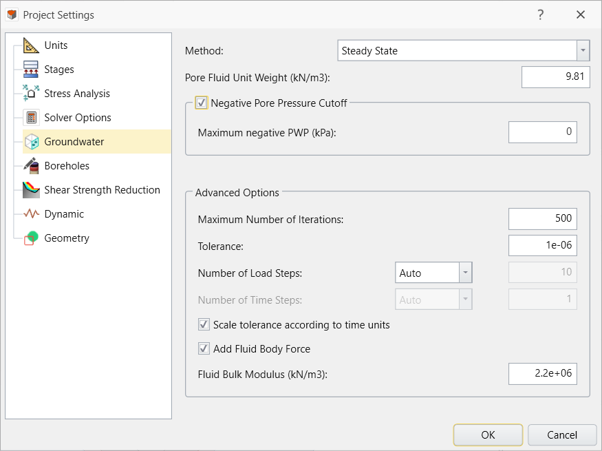

     

3. Leave the default settings for the rest of the parameters and click OK

3.0 Defining the Materials 

Ensure the current workflow tab is set to Geology 

1. Select: Groundwater > Define Hydraulic Properties

   For the hydraulic models, there are pre-defined models available in RS3 for describing the permeability in the unsaturated zone as a function of matric suction. For example, for the Van Genuchten, the permeability above the phreatic surface is automatically determined by RS3 based on matric suction. You can click the Plot Function button to view the plot of permeability versus matric suction. Click the link for a detailed description of each hydraulic model parameter. For this tutorial, we will define a model for each of the materials with constant permeability to reduce the non-linearity of the model and get the results quicker. 
2. Select User-defined Models next to Hydraulic Model dropdown 

3. Input the following parameters:

   • Name: Loose Sand
   • WC Input Type: By Degree of Saturation 
   • Input the values shown in the table for Permeability:

   Matric Suction (kPa)	Permeability (meters/second)
   0	0.0001
   1	0.0001

   To add a row, click on the Insert row into grid above currently selected row button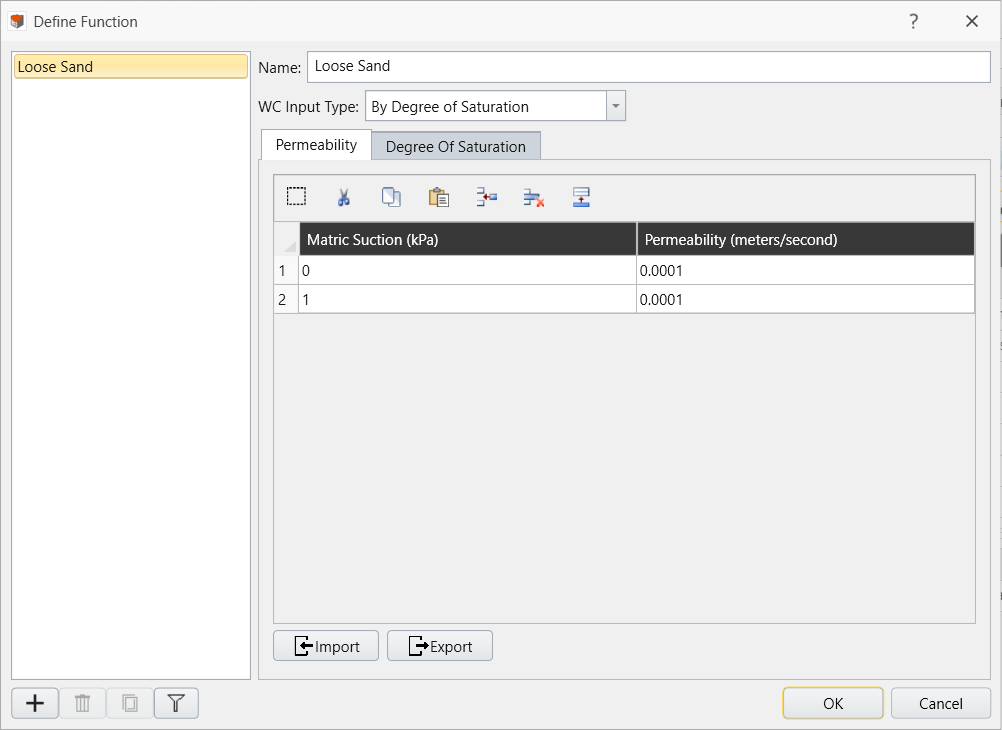

   

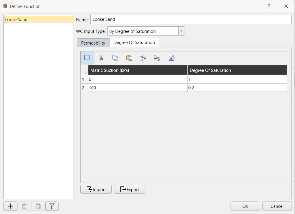
   • Switch to the Degree of saturation tab
   • Input the Values shown in the table for Degree Of Saturation:

   Matric Suction (kPa)	Degree Of Saturation
   0	1
   100	0.2

   

4. Click the Add new model button
   Input the following parameters:

   • Name: Clay
   • WC Input Type: By Degree of Saturation 
   • Input the values shown in the table for Permeability:

   Matric Suction (kPa)	Permeability (meters/second)
   0	1E-07
   1	1E-07

   • Input the Values shown in the table for Degree Of Saturation:

   Matric Suction (kPa)	Degree Of Saturation
   0	1
   100	0.2

5. Add a new model and input the following parameters:

   • Name: Dense Sand
   • WC Input Type: By Water Content 
   • Input the values shown in the table for Permeability:

   Matric Suction (kPa)	Permeability (meters/second)
   0	1E-06
   1	1E-06

   • Input the Values shown in the table for Water Content:

   Matric Suction (kPa)	Water Content (m3/m3)
   0	0.3
   100	0.2

    

6. Click OK to save and close the Define Function dialog

7. Select Loose Sand, change the Hydraulic Model to Loose Sand

   

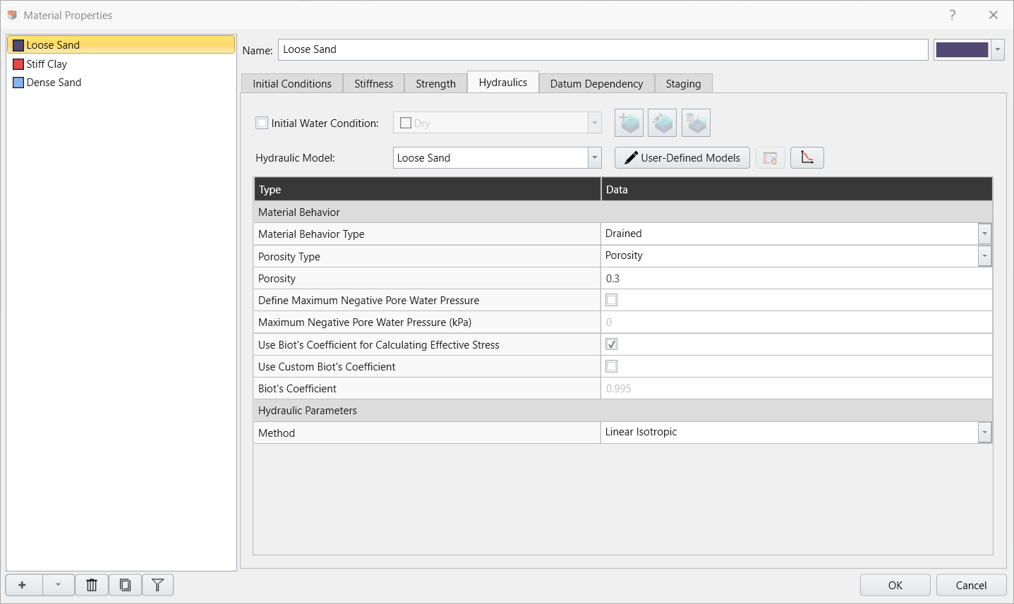
8. Select Stiff Clay, change the Hydraulic Model from Simple to Clay
9. Select Dense Sand, change the Hydraulic Model from Simple to Dense Sand
10. Click OK to save and close the Material Properties dialog
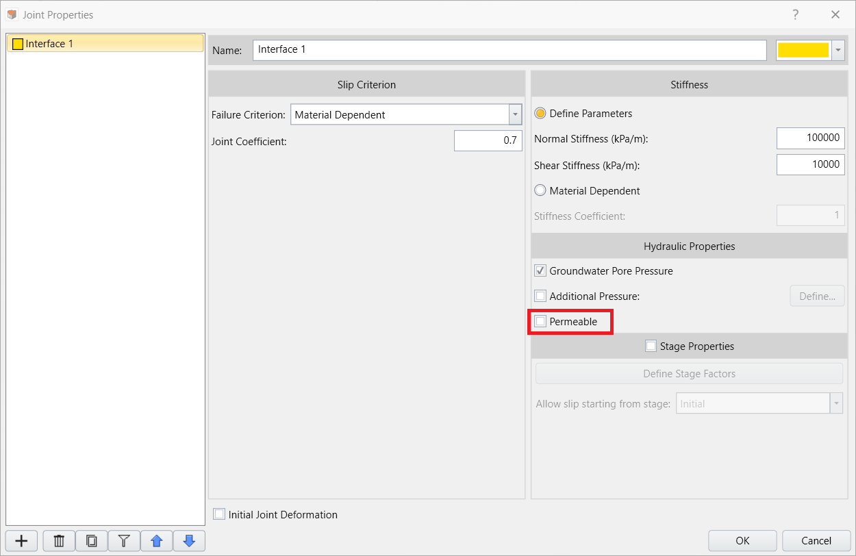
11. Select: Materials > Joints > Define Joint Properties

12. Uncheck Permeable under Hydraulic Properties

    This makes the walls surrounding the excavation impermeable, preventing water from flowing through the walls.

    

13. Click OK

4.0 Applying Groundwater Boundary Conditions

Set the current workflow tab to Groundwater

1. Select: Groundwater > Define Groundwater Boundary Conditions
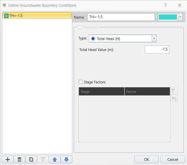
   Input the following parameters:
   • Name: TH=-1.5
   • Type: Total Head (H)

   • Total Head Value(m): -1.5

     

2. Click the Add new property button
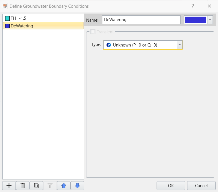
   Input the following parameters:
   • Name: DeWatering

   • Type: Unknown (P=0 or Q=0)

     

3. Click OK
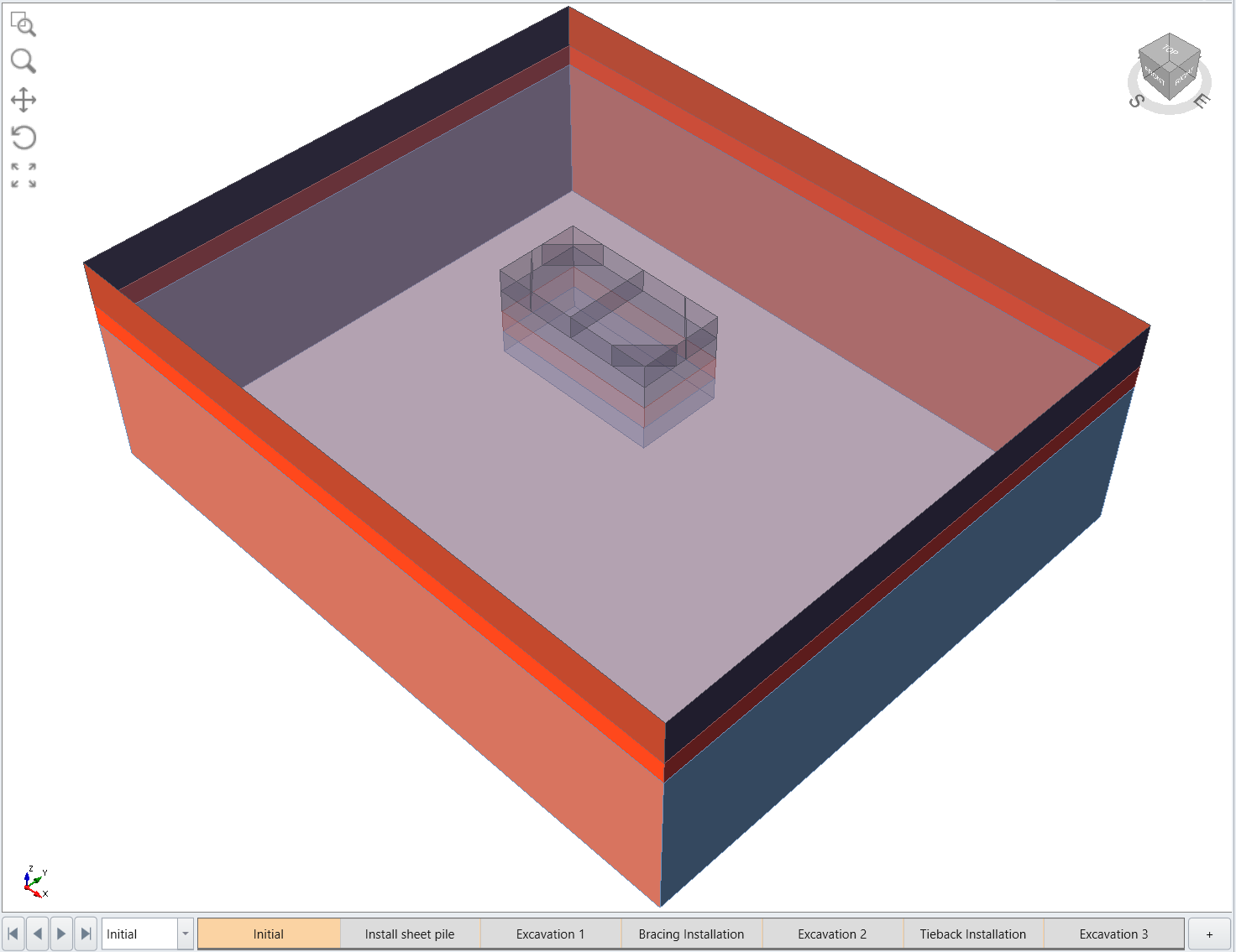
4. Select Initial stage 
5. Select Faces Selection

6. Select all the side faces of the intermediate entities:

   

7. Select Groundwater > Add Groundwater Boundary Conditions
   Input the following parameters:
   • Groundwater Boundary Condition: TH=-1.5
   • Install at stage: Initial 

   • Remove at stage: Never

     

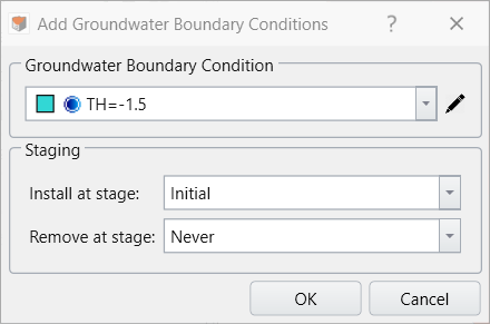
8. Click OK

   

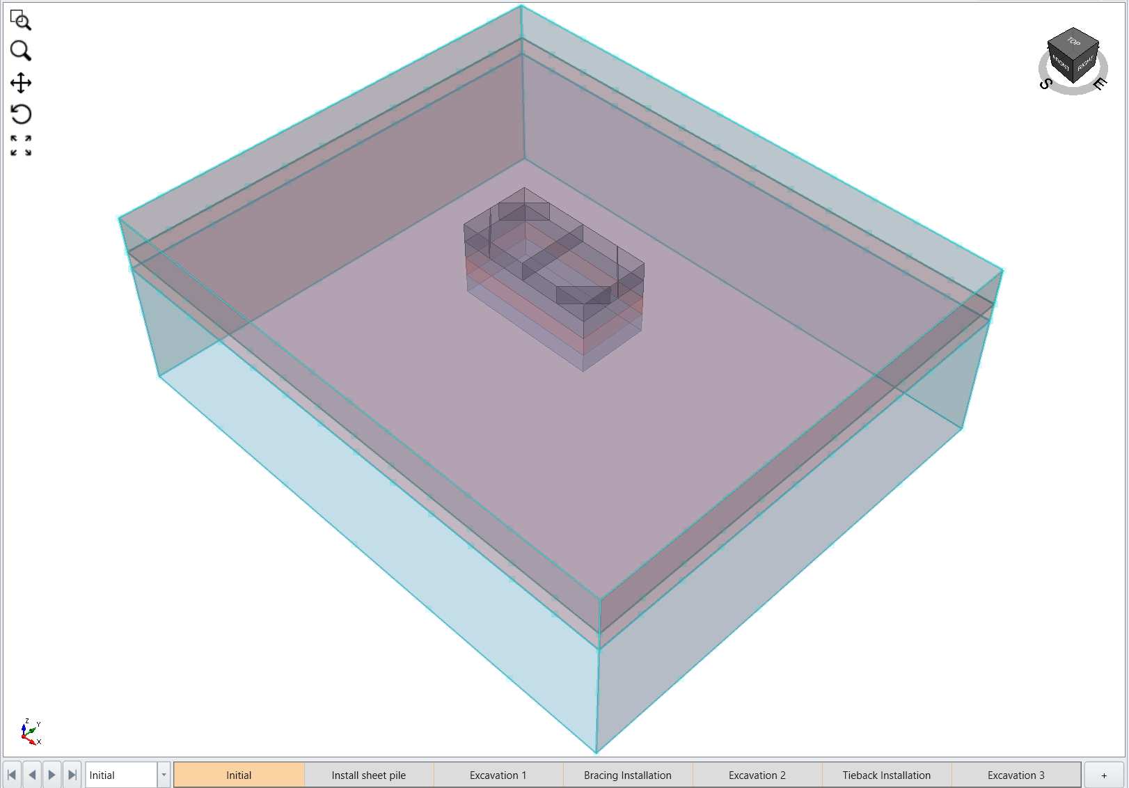
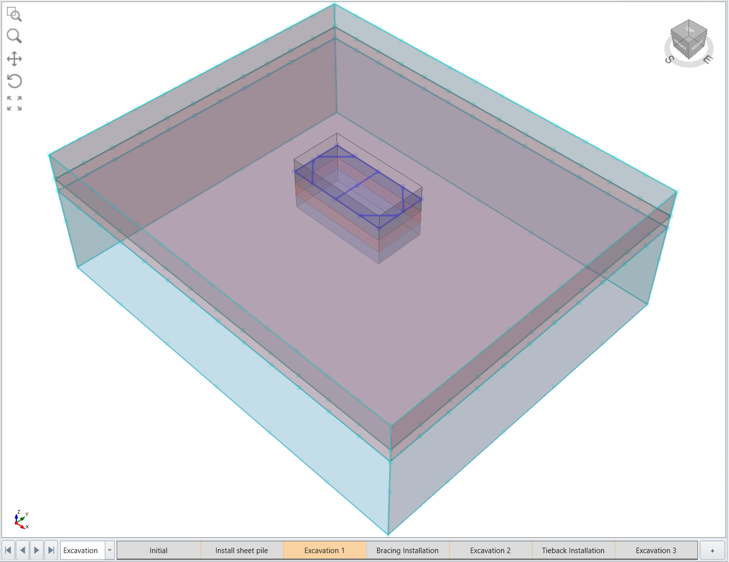
9. Select Excavation 1 stage
10. Hide the top layer box entities

11. Select the faces at the bottom of the first excavation 

    

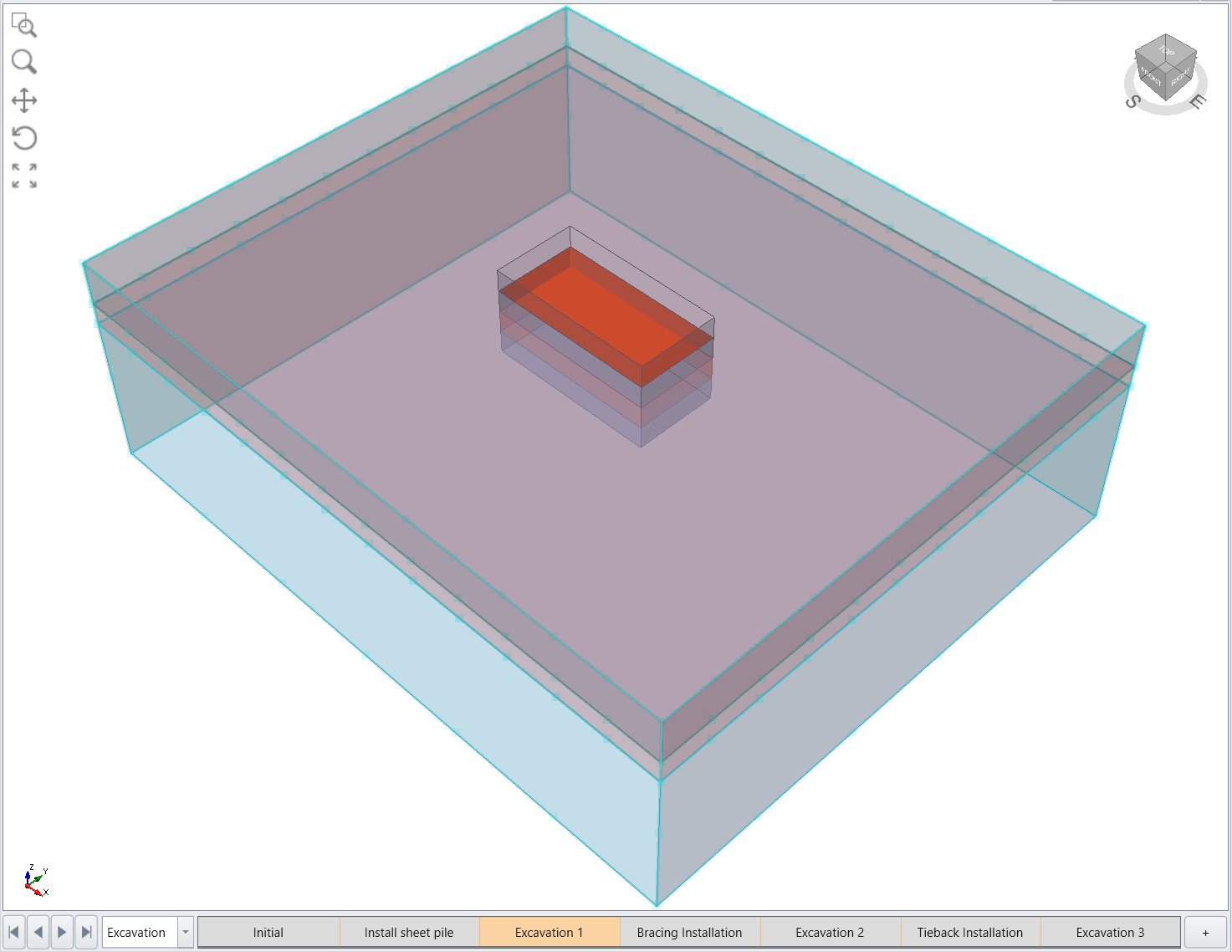
12. Select Groundwater > Add Groundwater Boundary Conditions
    Input the following parameters:
    • Groundwater Boundary Condition: DeWatering
    • Install at stage: Excavation 1 

    • Remove at stage: Excavation 2

      

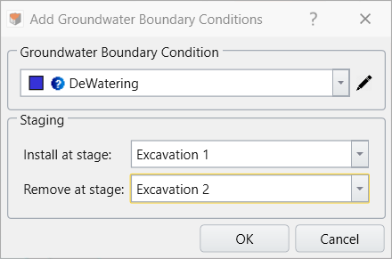
13. Click OK

    

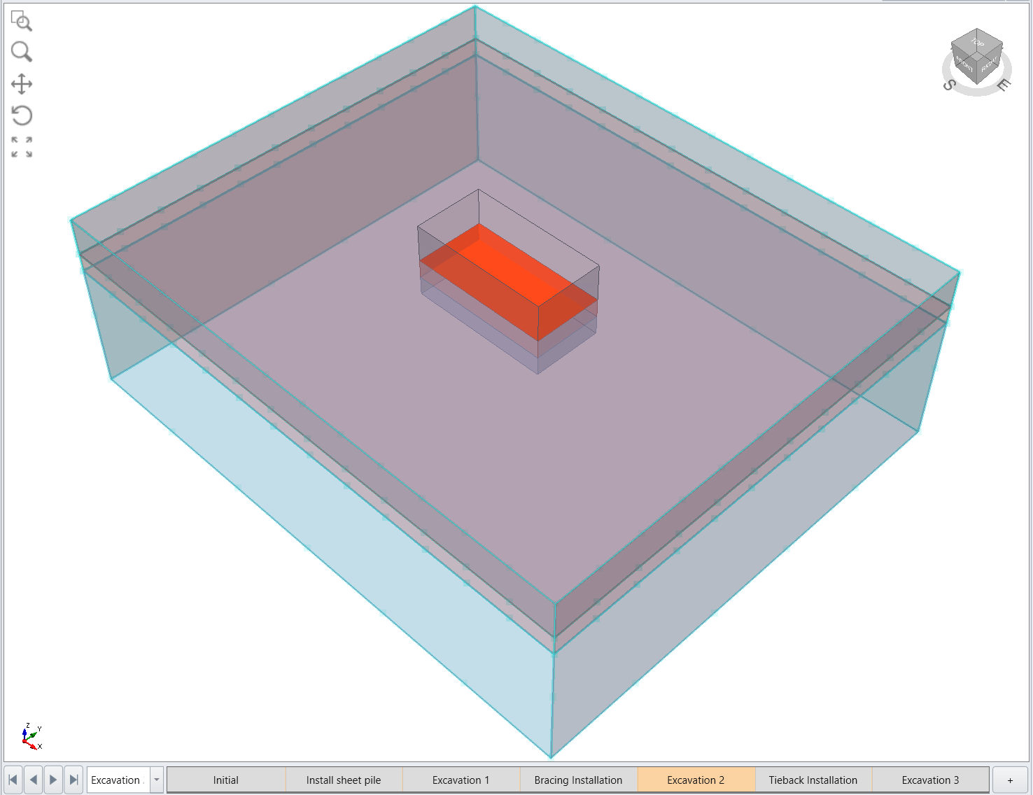
14. Select Excavation 2 stage
15. Hide the second layer from the top box entity

16. Select the face at the bottom of the second excavation 

    

17. Select Groundwater > Add Groundwater Boundary Conditions

    Input the following parameters:

    • Groundwater Boundary Condition: DeWatering
    • Install at stage: Excavation 2

    • Remove at stage: Excavation 3

      

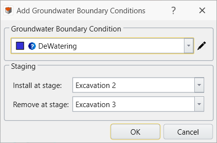
18. Click OK

    

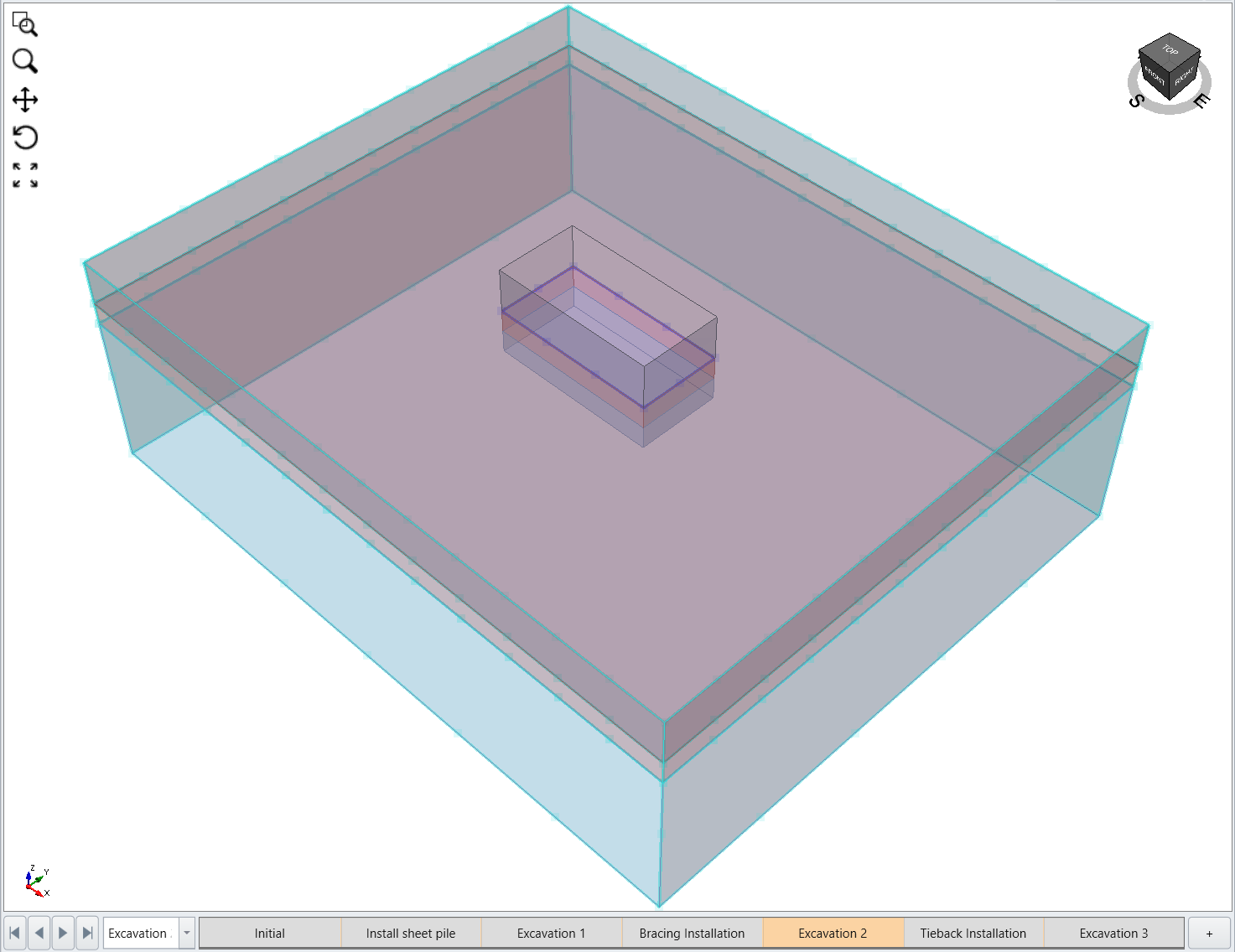
19. Select Excavation 3 stage
20. Hide the third layer from the top box entity 

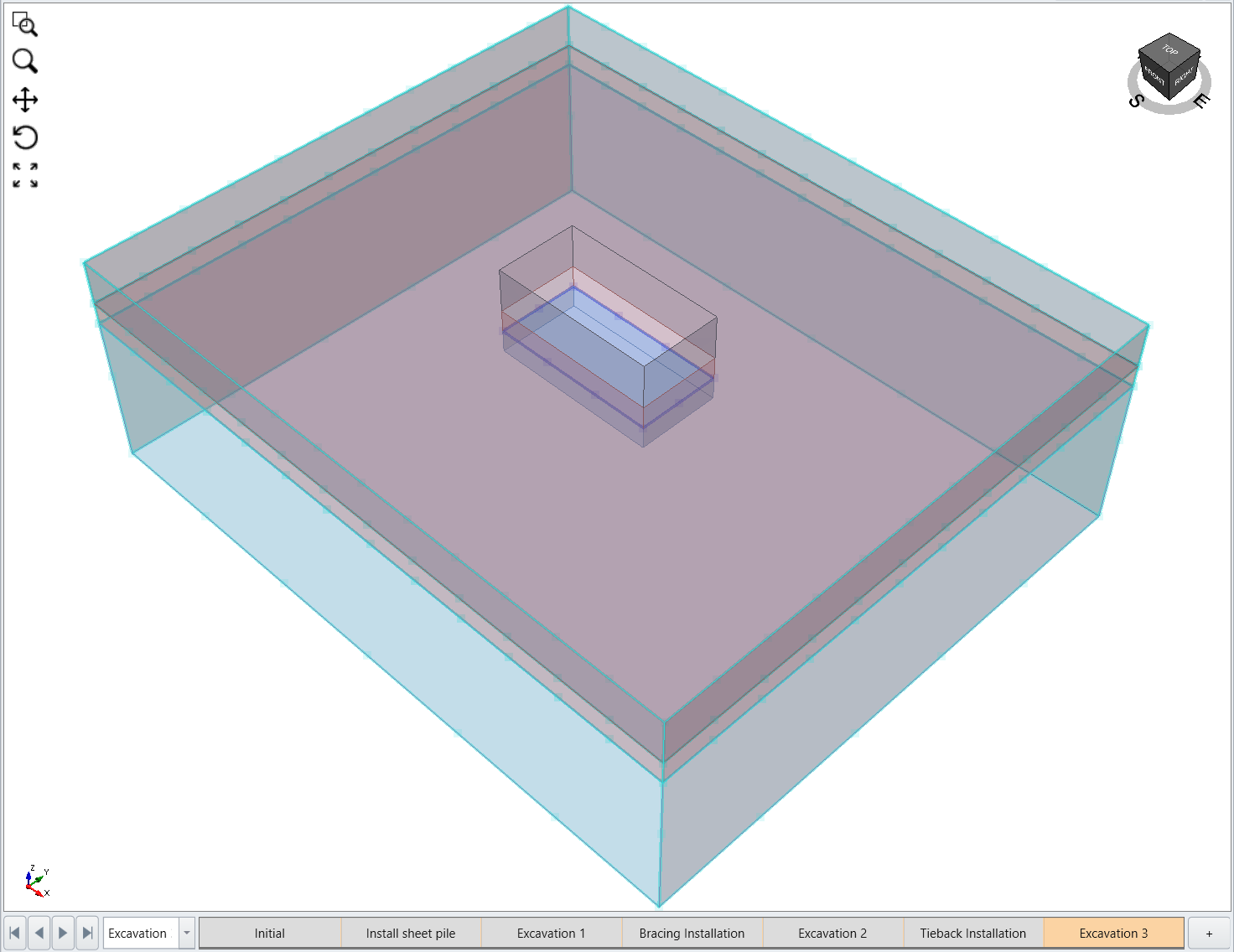
21. Select the bottom face of the third excavation 

    

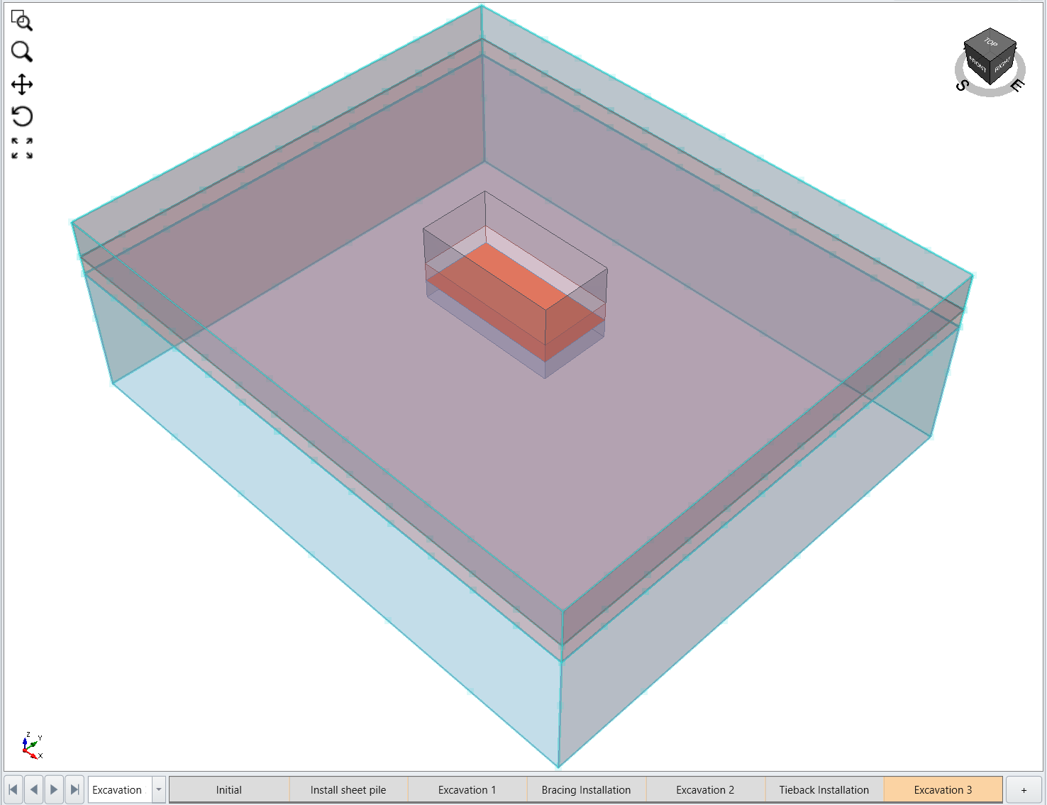
22. Select: Groundwater > Add Groundwater Boundary Conditions
    Input the following parameters:
    • Groundwater Boundary Condition: DeWatering
    • Install at stage: Excavation 3

    • Remove at stage: Never

      

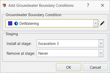
23. Click OK

    

5.0 Restraints

Set the current workflow tab to Restraints

1. Select: Restraints > Reset All Displacements 
2. Make sure Reset Displacements after stages:  is selected

3. Leave the stage as Initial 

   

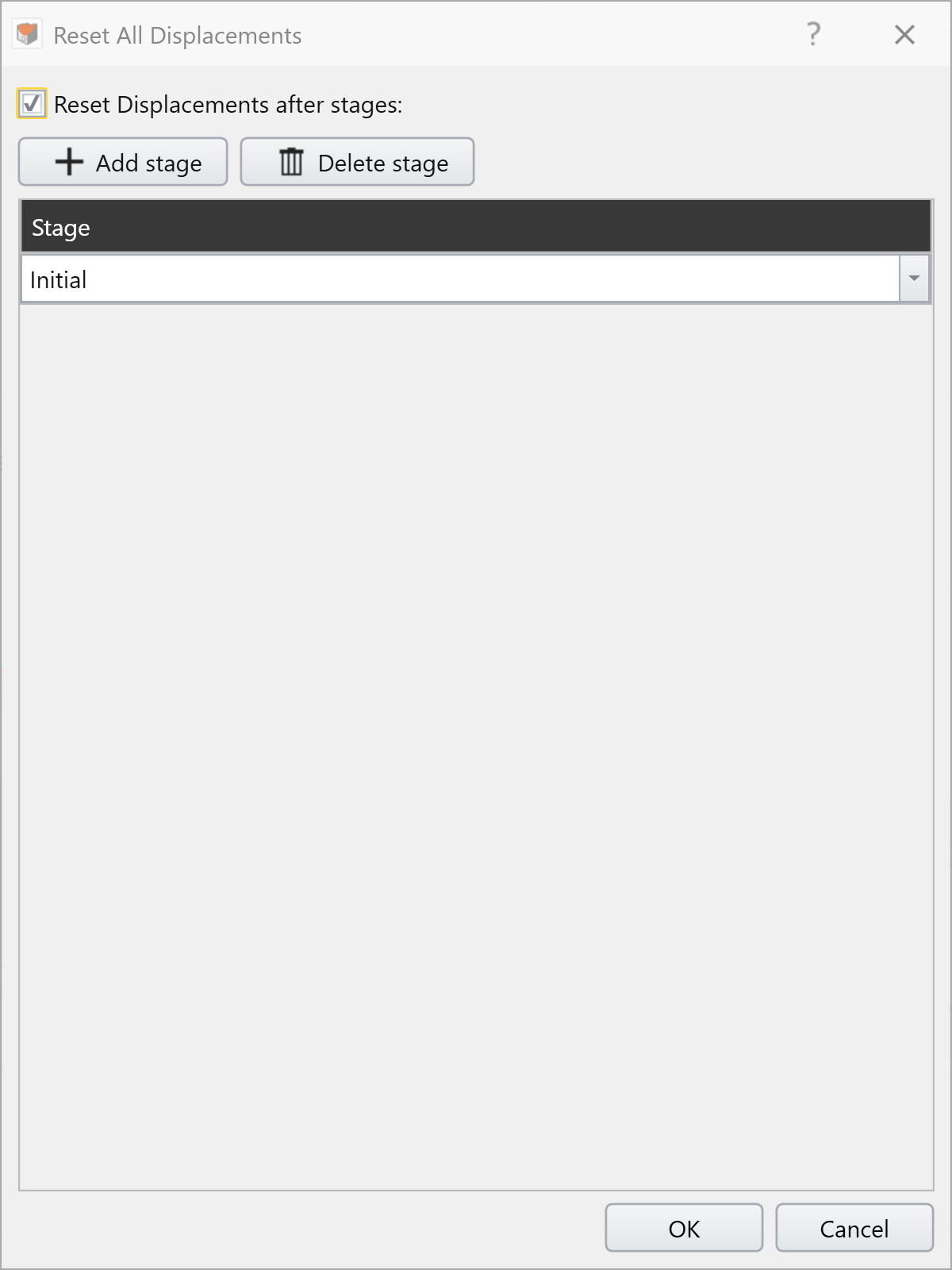
4. Select OK

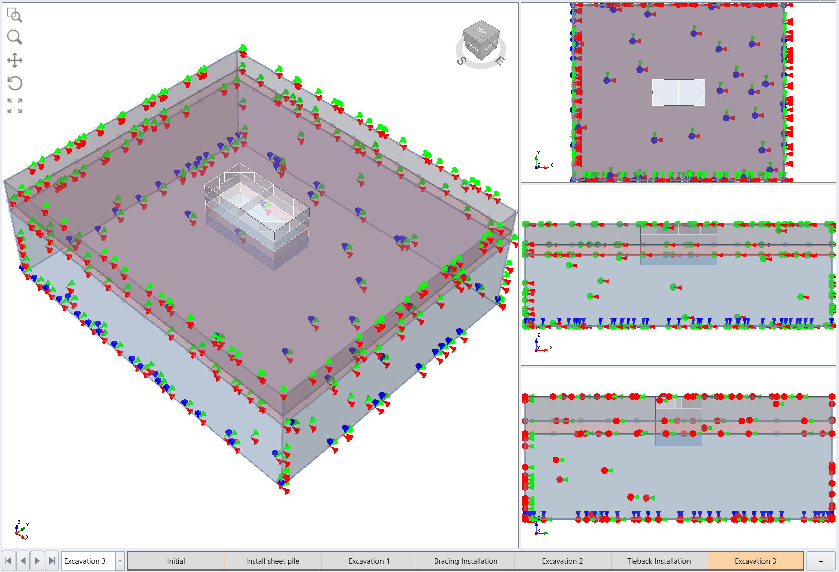
5. Select: Restraints > Auto Rotation Restrain (Surface)

   

6.0 Mesh

Set the current workflow tab to Mesh

1. Select Mesh > Mesh Settings

   

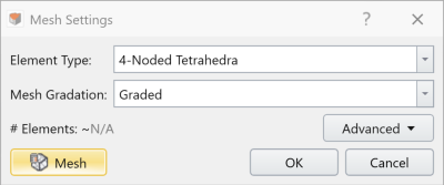
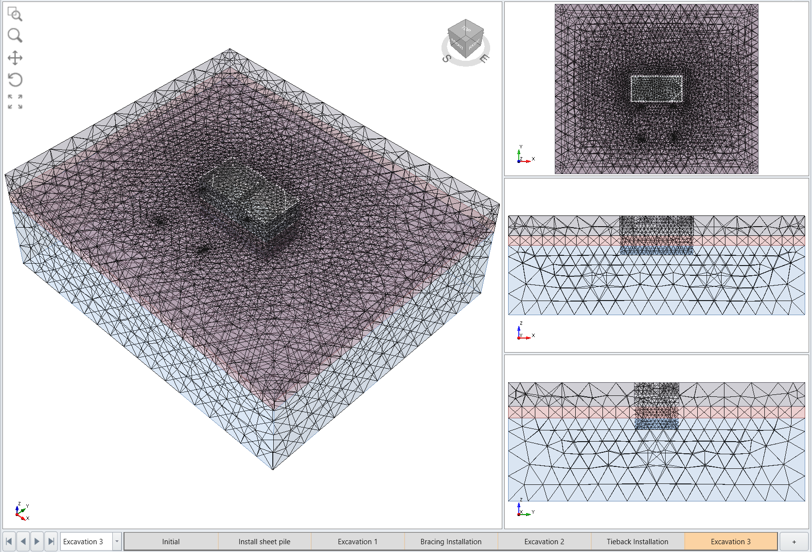
2. Keep the default settings and select Mesh

3. Click OK

   

7.0 Compute

Set the current workflow tab to Compute

1. It is recommended to save the final model as a separate file so that you can access the original file anytime: File > Save As
2. Select Compute > Compute

You can compute only groundwater by selecting Compute > Compute (Groundwater Only)

8.0 Results 

Set the current workflow tab to Results

8.1 GROUNDWATER RESULTS

8.1.1 Pressure Head

1. Select Excavation 3 stage
2. On the top right corner, set the Legend to Solids and Pressure Head

3. Select Interpret > Show Data on Plane > XZ
   Leave default parameters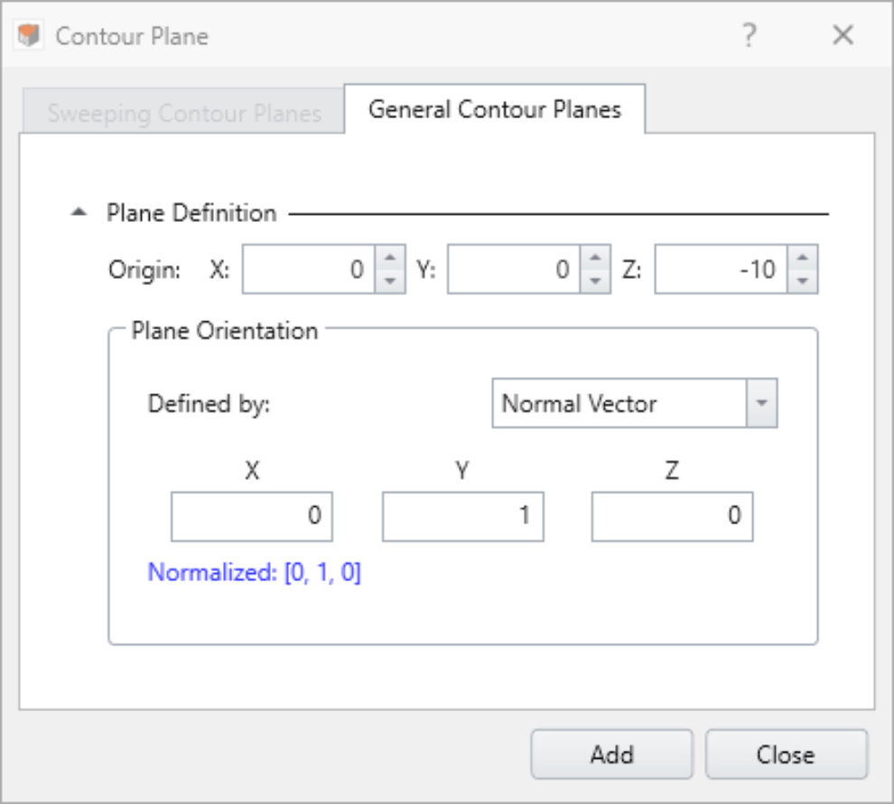

   

   

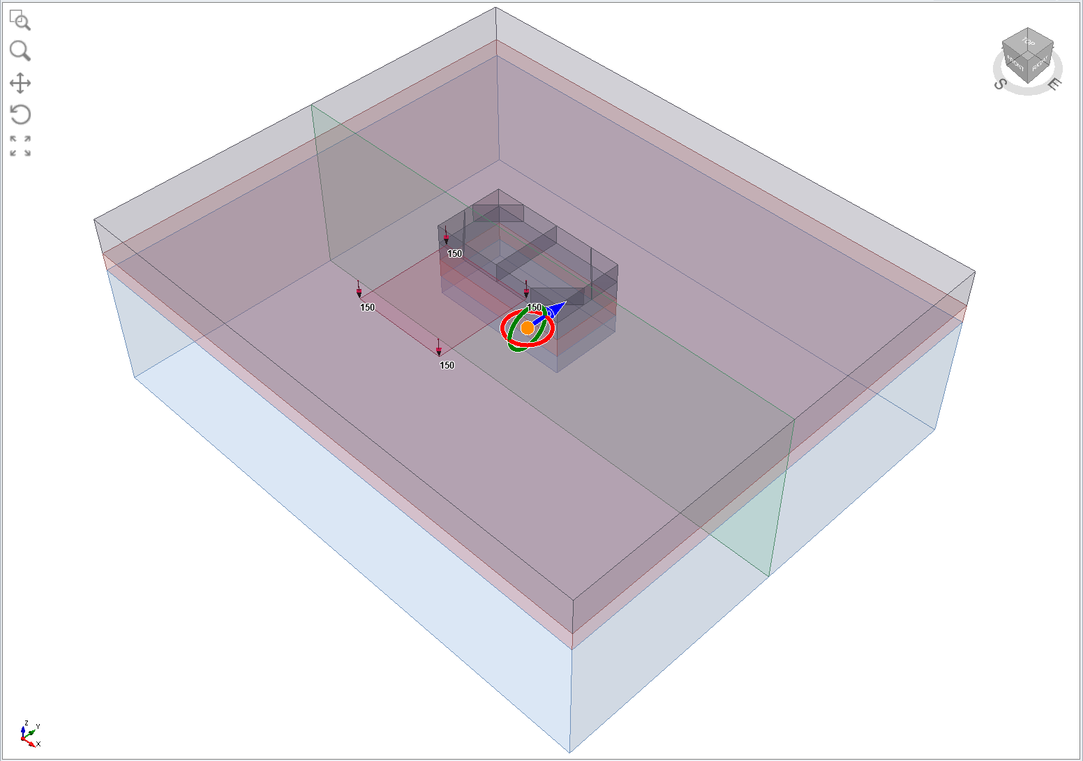
4. Click Add
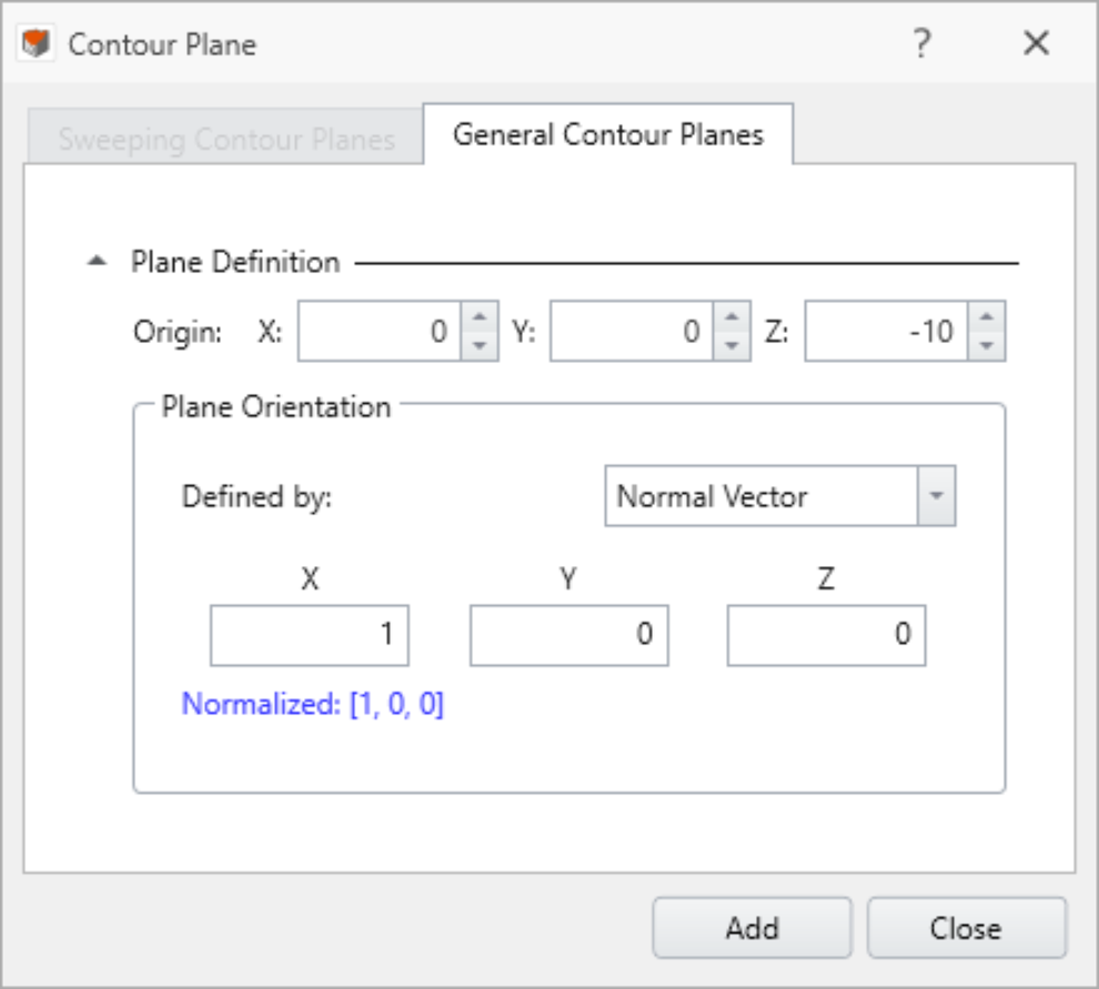
5. Adjust the plane orientation to (1, 0, 0)

6. Click Add and close the dialog

   

   

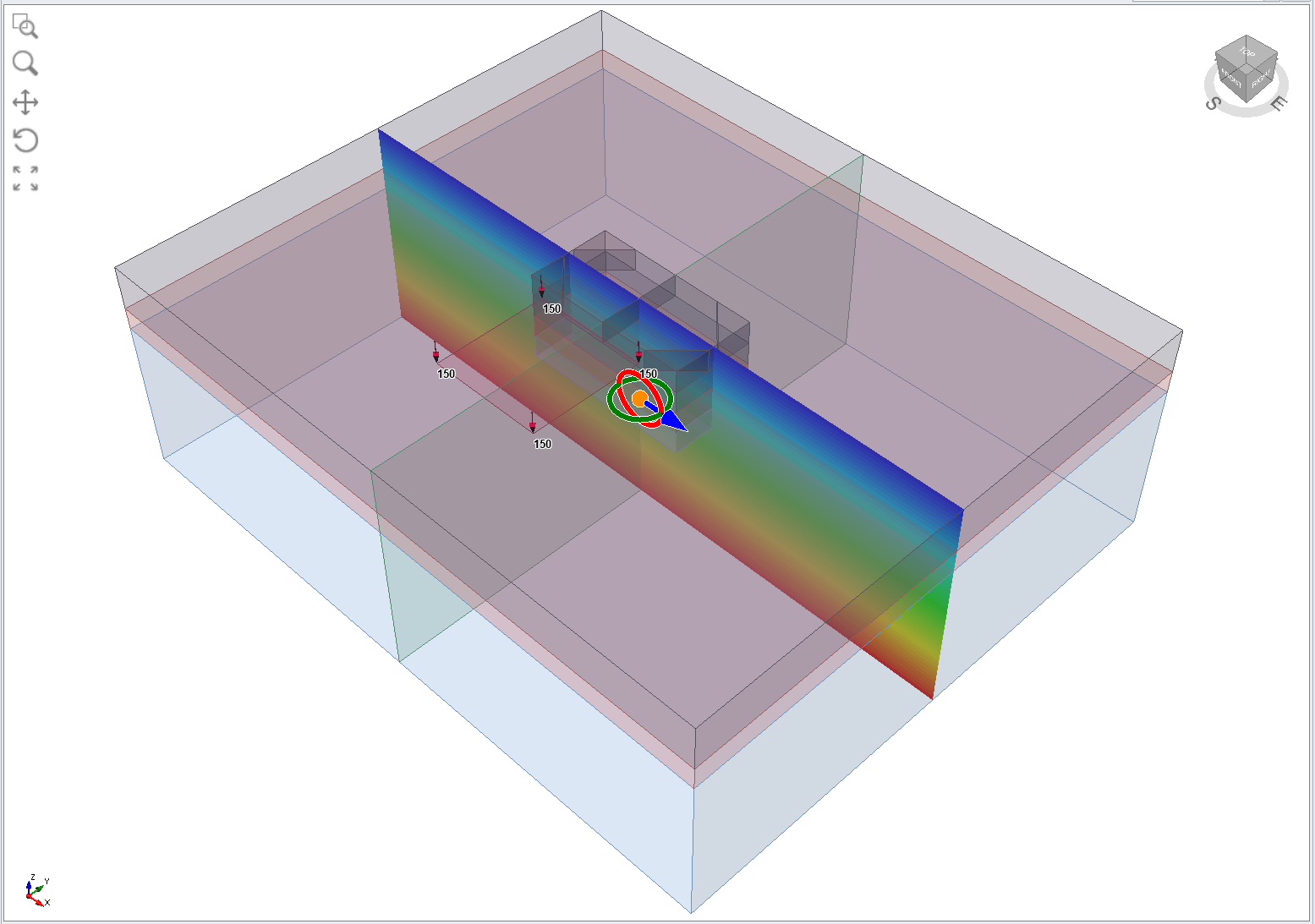
7. Select: Interpret > Contour Legend > Contour Options
   Input the following parameters:
   • Custom Range: 0 to 18.5
   • Interval Count: 20

   • Check Show Contour Lines

     

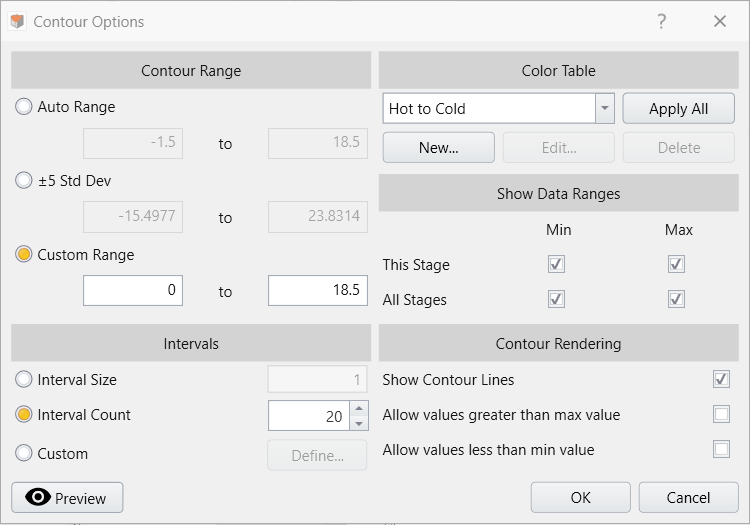
8. Click OK

   

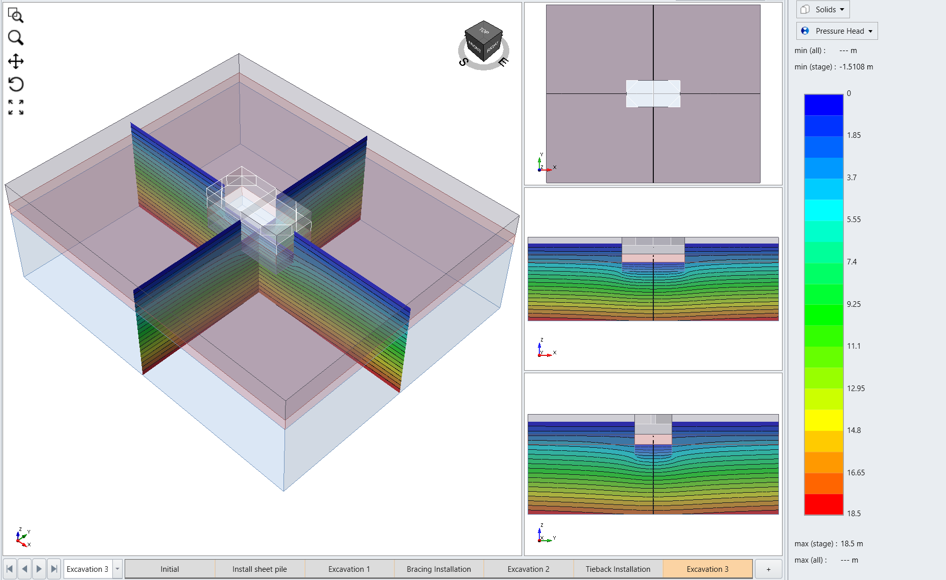
9. Select the YZ contour plane from the visibility tree
10. Right-click > Hide All But Selected Geometry 
11. Unhide the SheetPile Wall and SheetPile Wall 3 entities from the visibility tree
12. Below are the results for the Initial stage, Excavation 1 stage, Excavation 2 stage, and Excavation 3 stage from the right view

Initial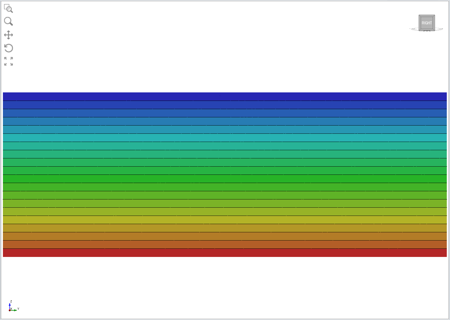
Excavation 1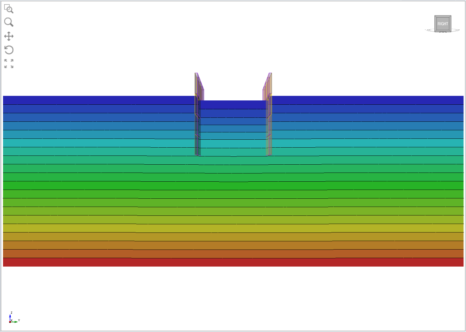
Excavation 2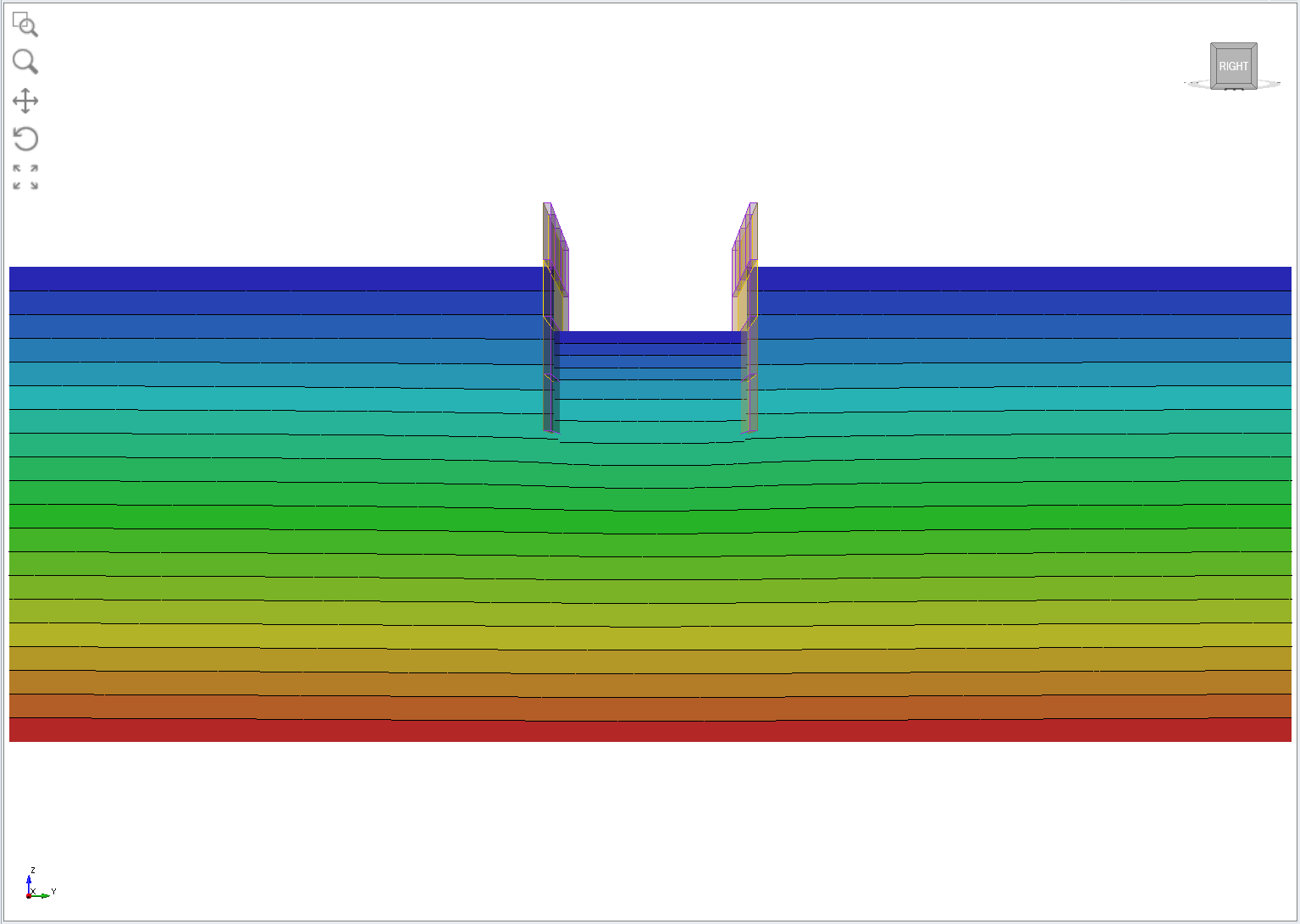
Excavation 3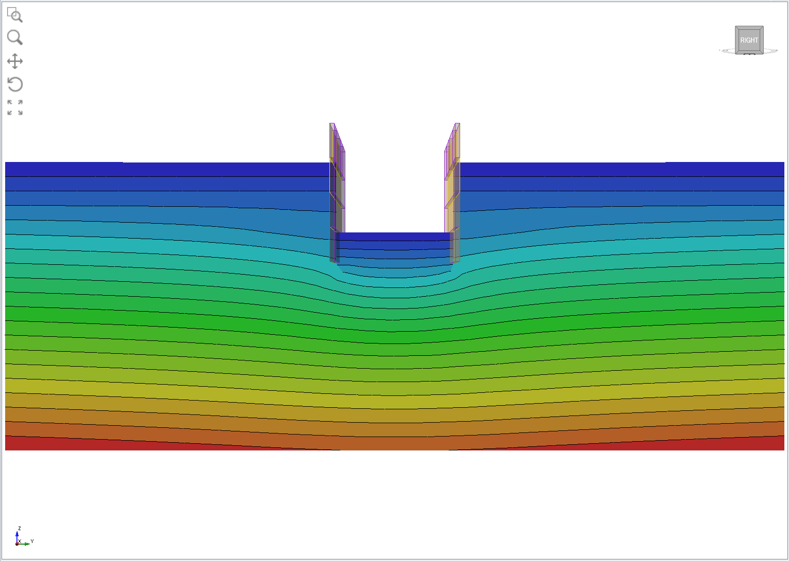

Since the wall is impermeable, the pore pressure in the soil on either side of the wall is discontinuous as shown in the images above.

8.1.2 FLUID FLOW

1. Show only the excavation and external volumes from the visibility tree
2. Select Excavation 3 stage
3. Select: Interpret > Queries > Add Fluid Flow Query 
   Input the following coordinates (press Enter after each input):
   (0, -10, -1) 
   (0, -10, -8)

4. Right-Click > Done
   In the Fluid Flow Query Options dialog, select the first option and input 5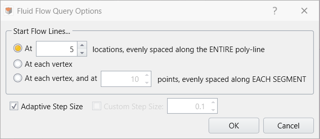

   

5. Click OK

6. Repeat steps 3 to 5 to create three more fluid flow queries with the following coordinates:
   (0, 10, -1) and (0, 10, -8)
   (-12, 0, -1) and (-12, 0, -8)
   (12, 0, -1) and (12, 0, -8)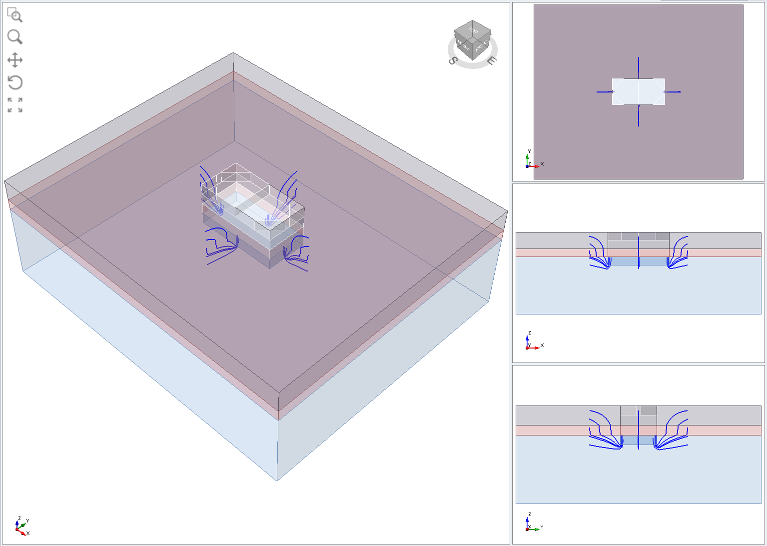

   

7. Below are the results for Excavation 1 stage and Excavation 2 stage

   

   

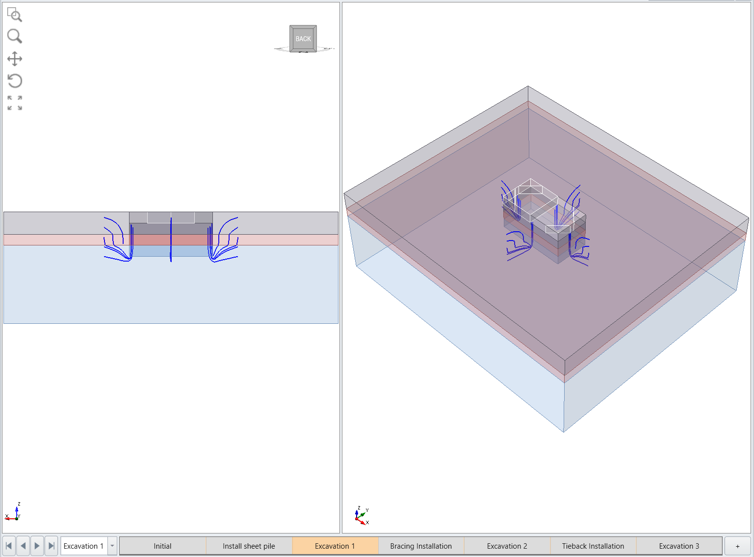
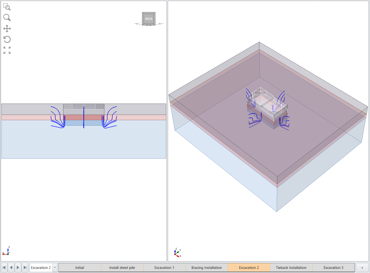
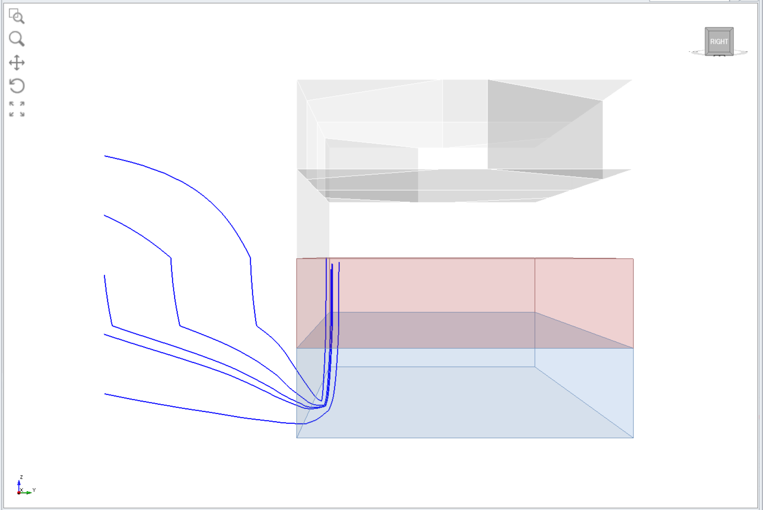
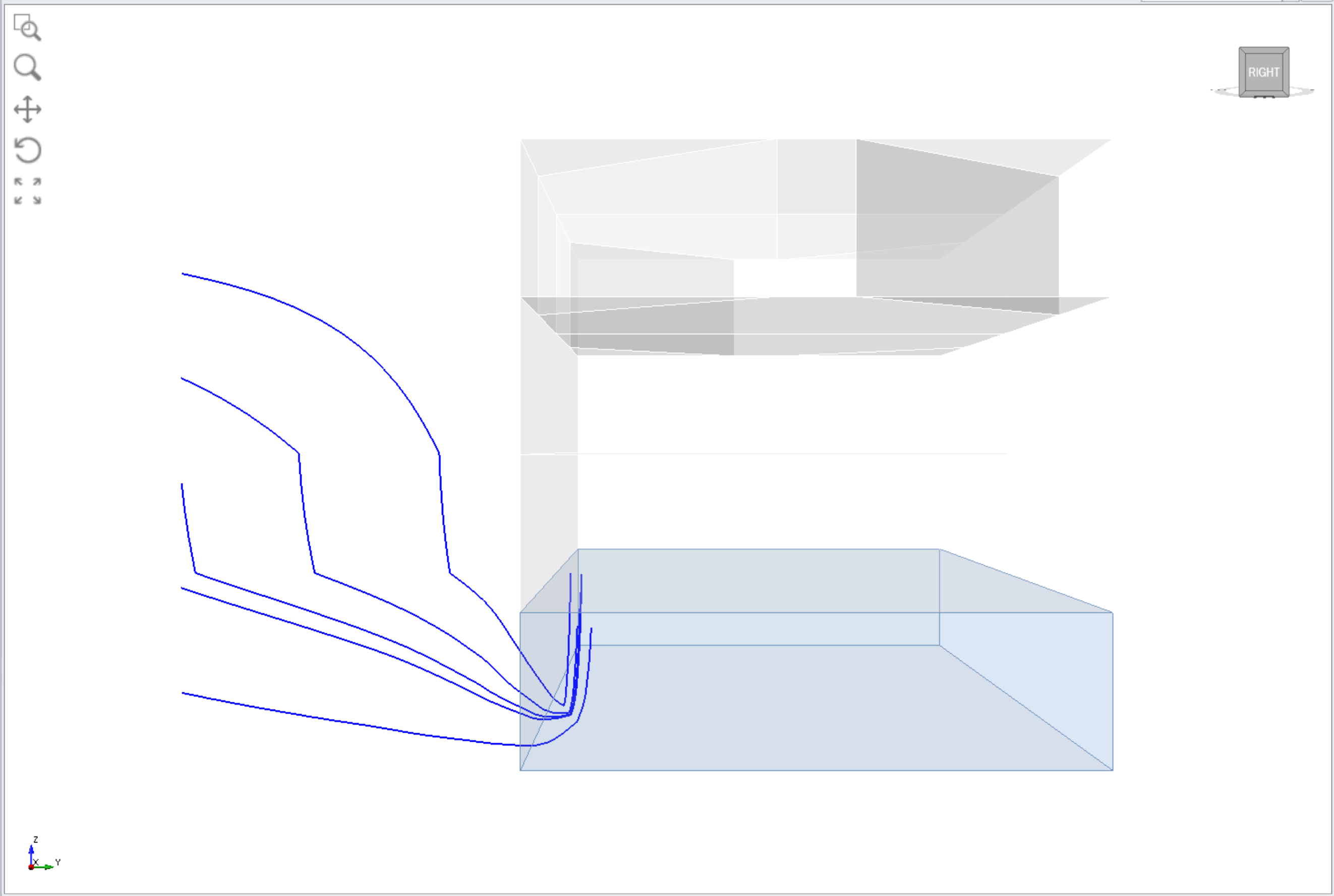
8. Below are the results of the fluid flow from the right view

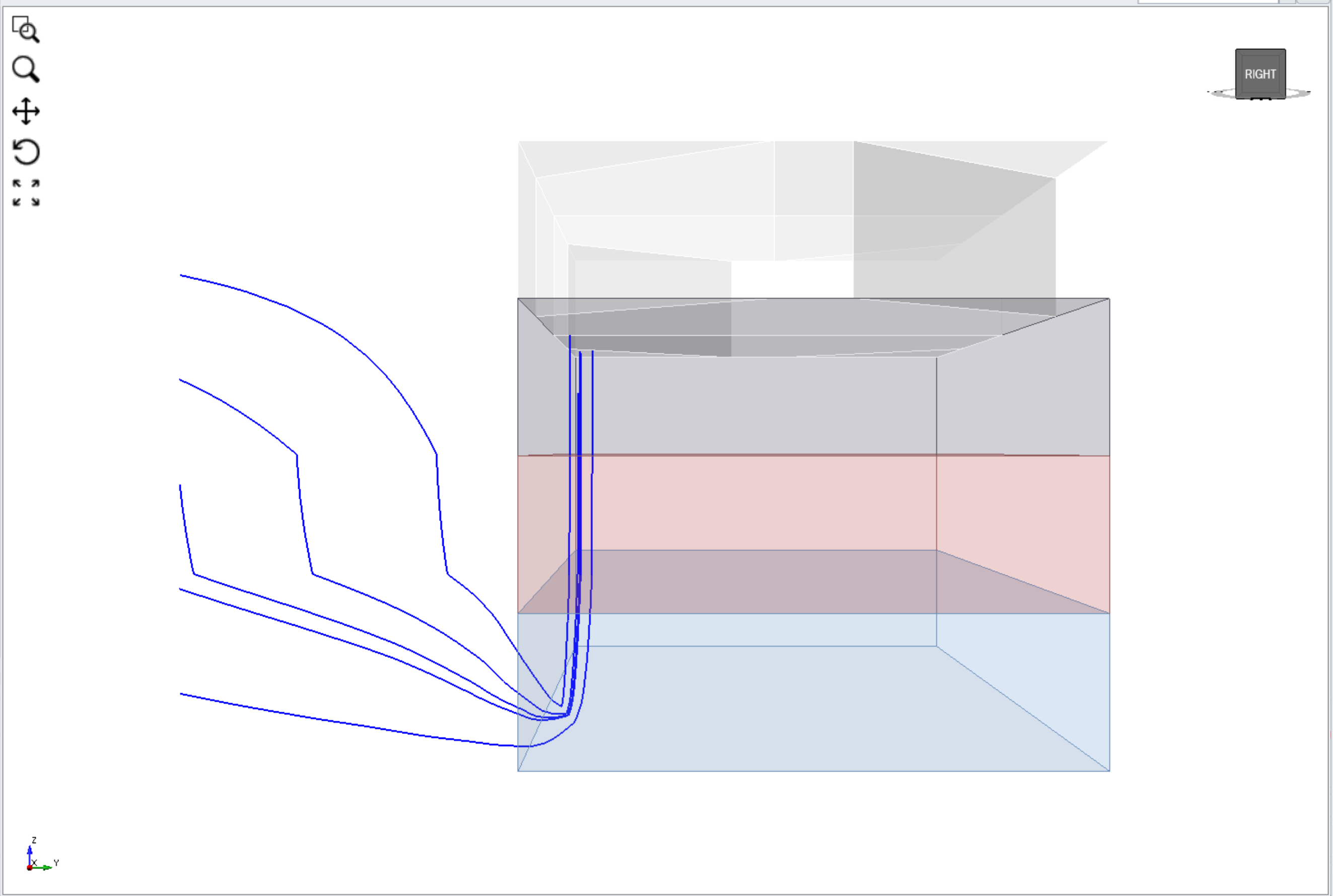
   Excavation 1	Excavation 2	Excavation 3

8.2 COMPARISON WITH THE DRY CASE

8.2.1 EXCAVATION RESULTS

1. Hide the fluid flow 
2. Select Excavation 3 stage
3. On the top right corner, set the Legend to Solids and Total Displacement 
4. Unhide the contour planes
5. Select: Interpret > Show Excavation Contour 
6. Select all external volume entities from the Visibility Tree

7. Adjust the transparency higher from the properties pane to visualize the displacement distribution more clearly

   

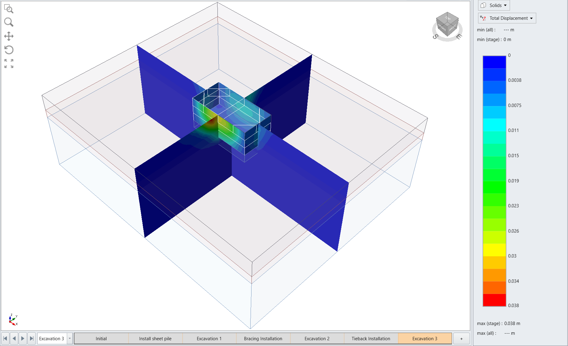
   Result from previous dry case:

   

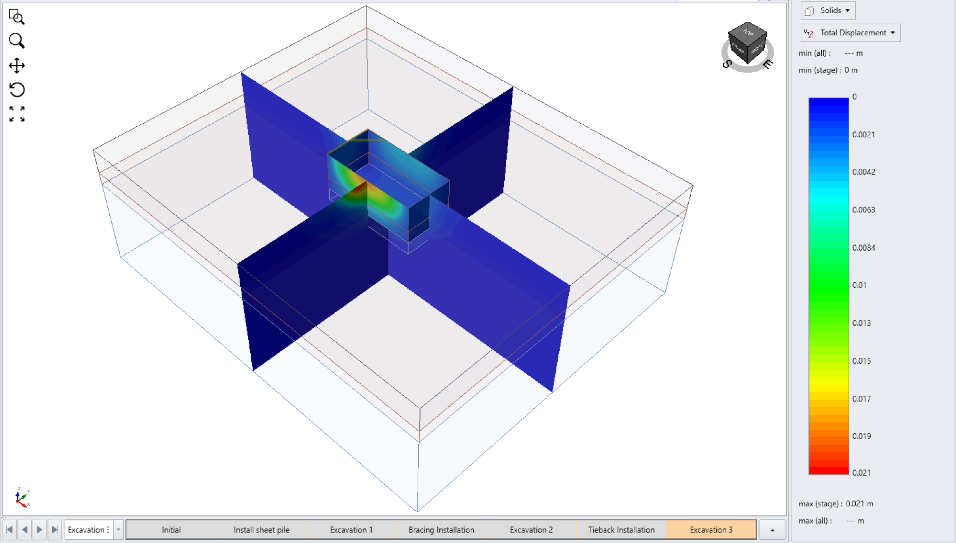
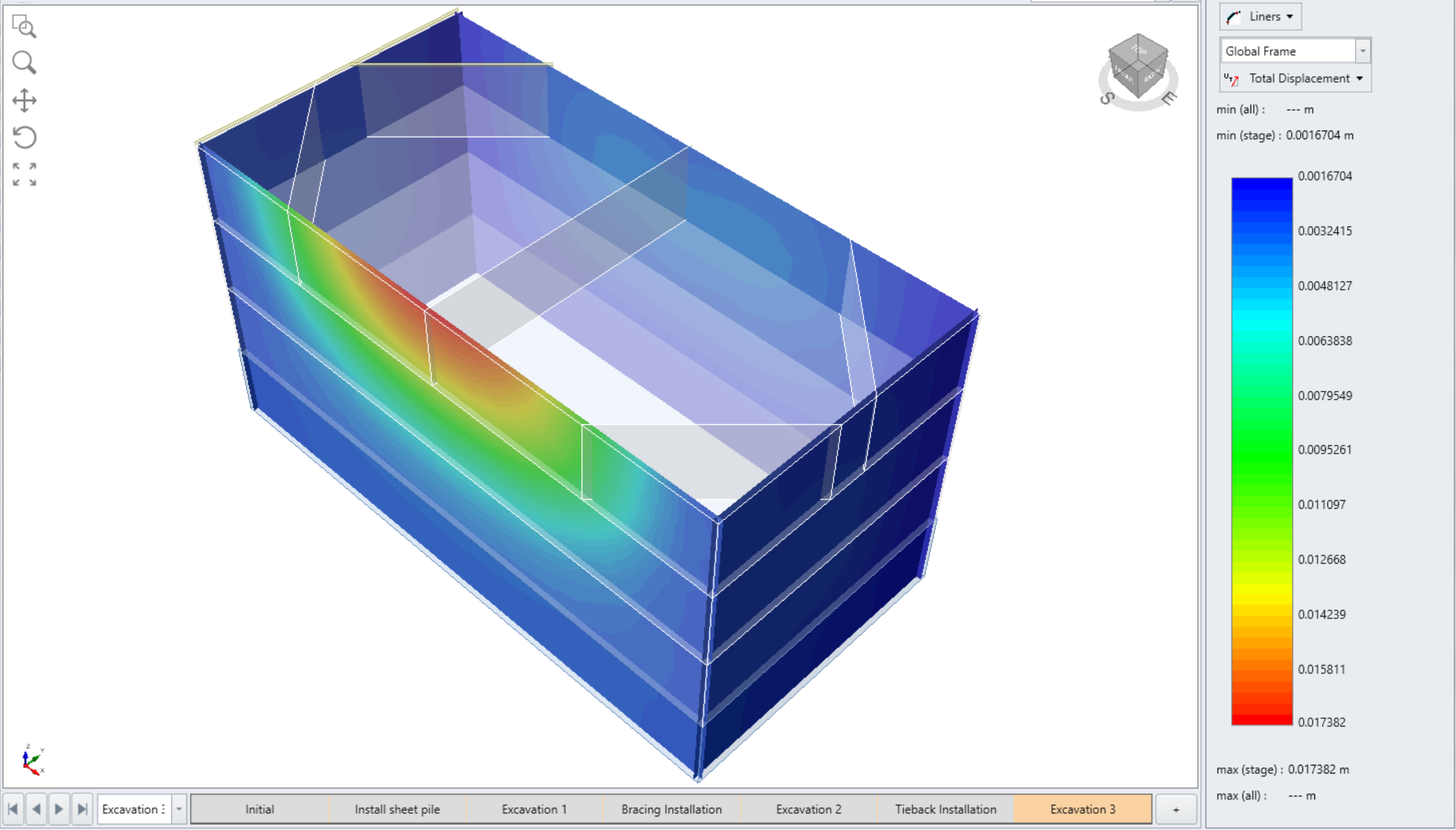
Displacement is slightly higher in the wet case due to the water pressure that is applied to the wall.

8.2.2 BOLT RESULTS

1. Hide all entities from the visibility tree but the excavation volumes
2. Set the Legend to Bolts and Axial Force

3. Select Excavation 3 stage 

   

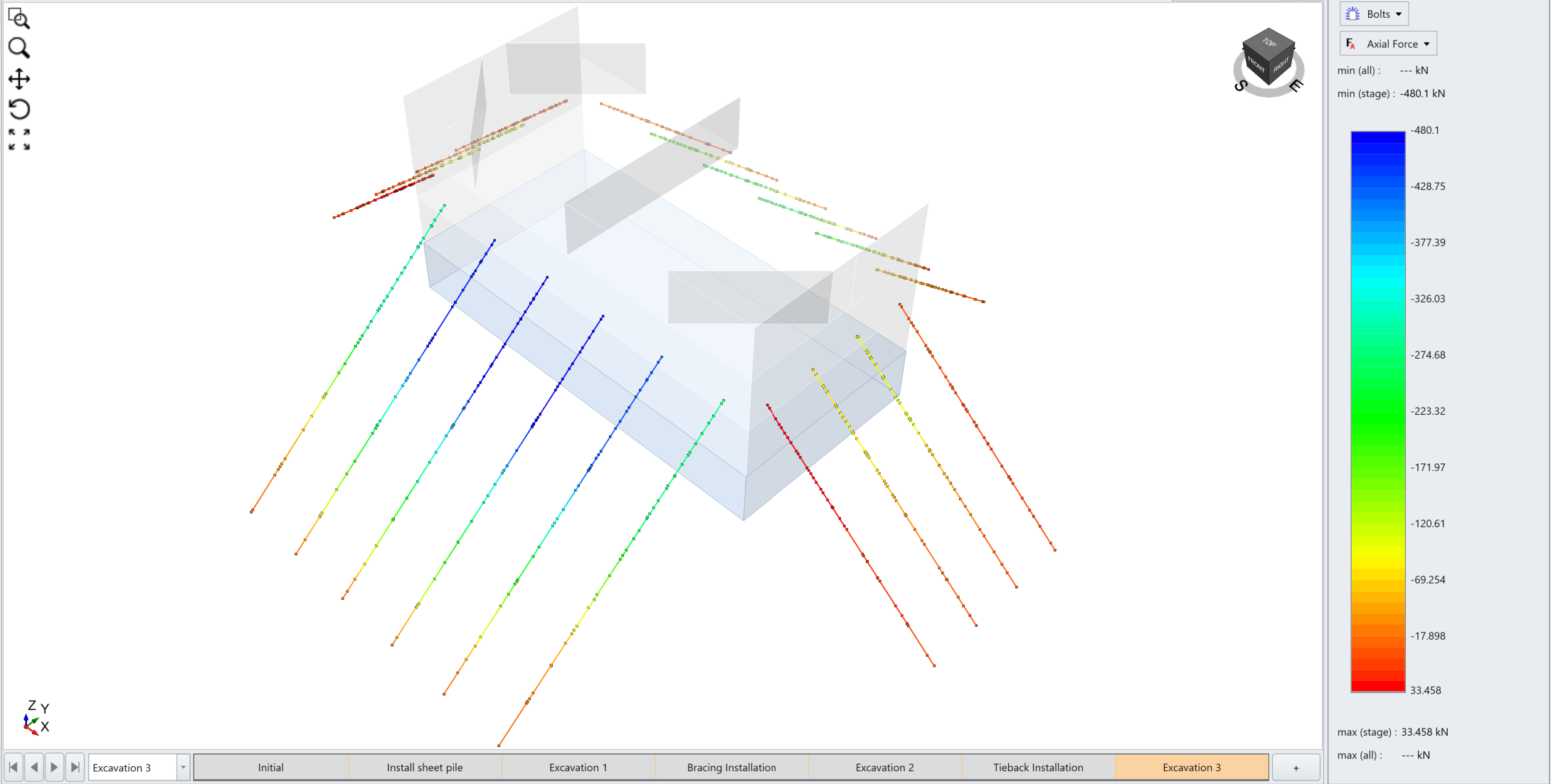
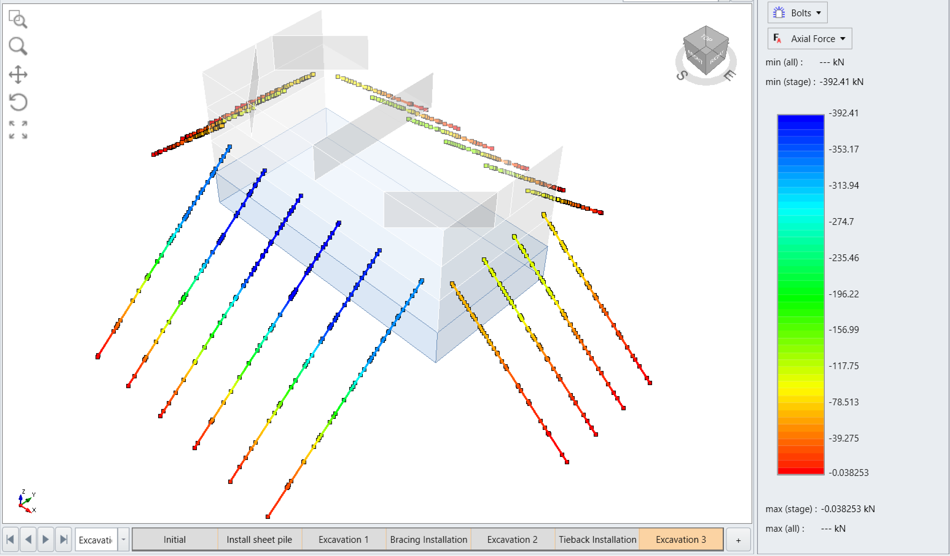
   Previous dry case:

   

4. Select Bolt 2: Pattern Results from the Visibility Tree then Select point 4 from the Properties Pane

5. Select Graph Data from the Properties Pane

   

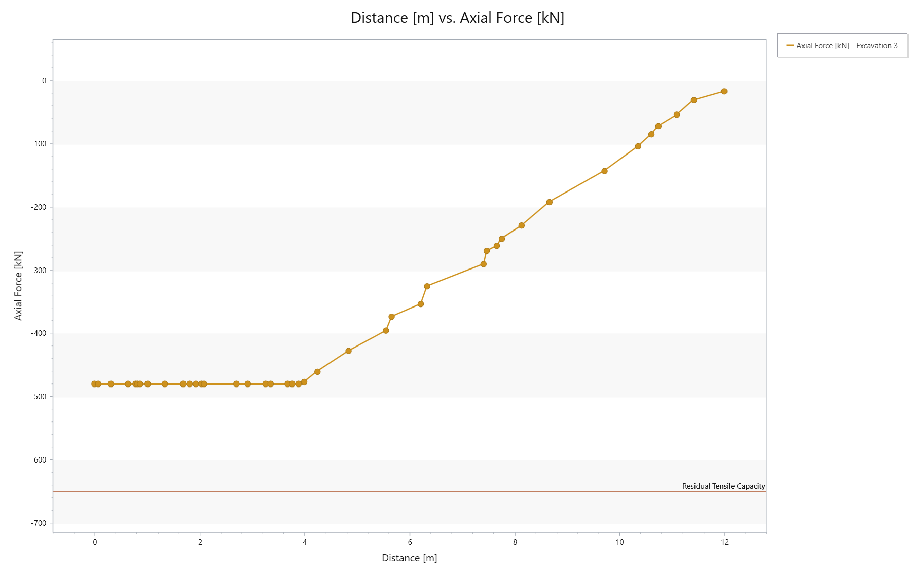
   Previous dry case:

   

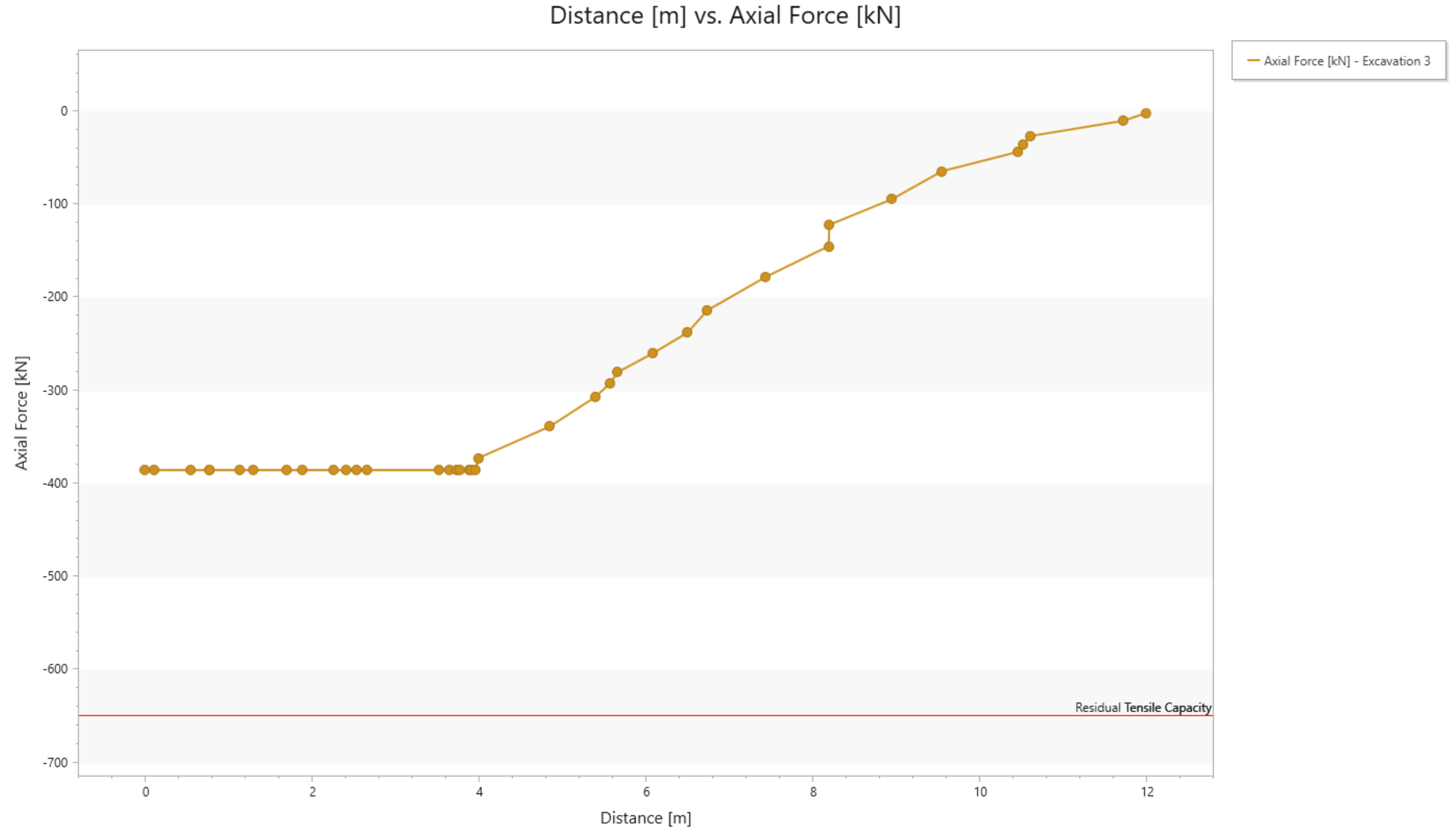
   The graph shows that the axial force increases in the wet case. This is due to the additional pore pressure that is applied to the wall.

8.2.3 WALL RESULTS

1. Set the Legend to Liners and Total Displacement

   

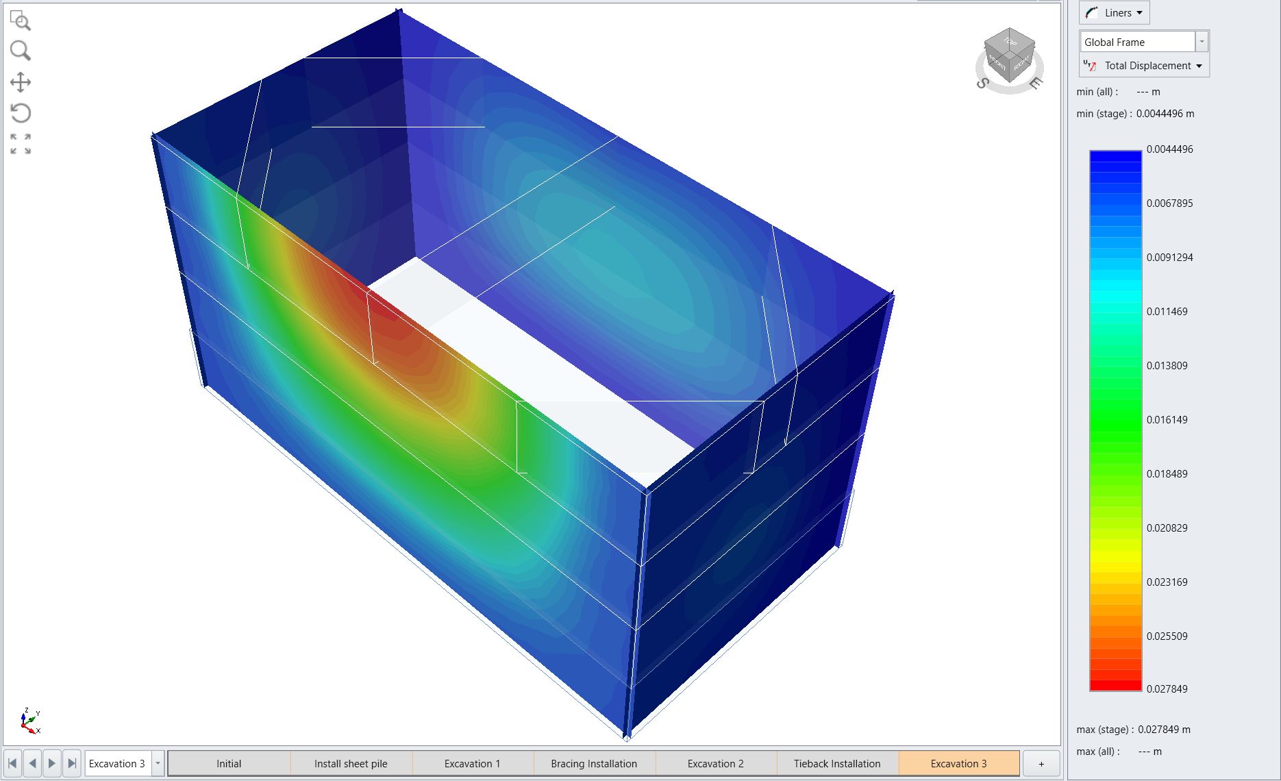
   Previous dry case:

   

2. Select SheetPile Wall from the Visibility Tree
3. Right-Click > Hide All But Selected Geometry
4. Select: Interpret > Queries > Add Liner Line Query To Surface
5. Select the mid-point on the top then select the mid-point on the bottom

6. Right-Click > Done

   

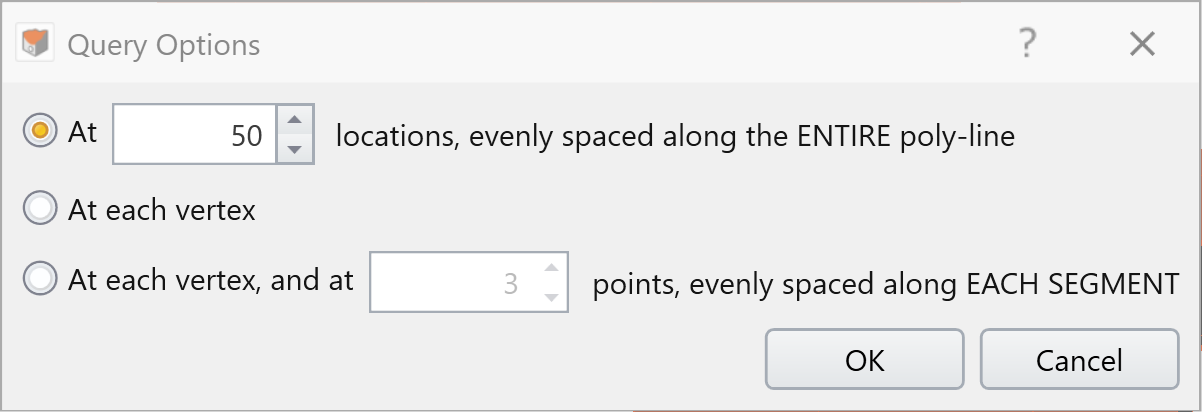
7. Click OK
8. Select the query line from the Visibility Tree
9. Select Graph Data from the Properties Pane
10. From the Chart Options, select Change Plot Data
    • Primary Data: Y Displacement [m]
    • Horizontal Axis: Distance [m]
    • Secondary Data: Excavation 1, Excavation 2, and Excavation 3
11. Click OK
12. From the Chart Options select,
    • Swap Axes
    • Reverse X-Axis
    • Reverse Y-Axis
    • Min X Value: 0
    • Max X Value: 8
    • Min Y Value: 0

    • Max Y Value: 0.05

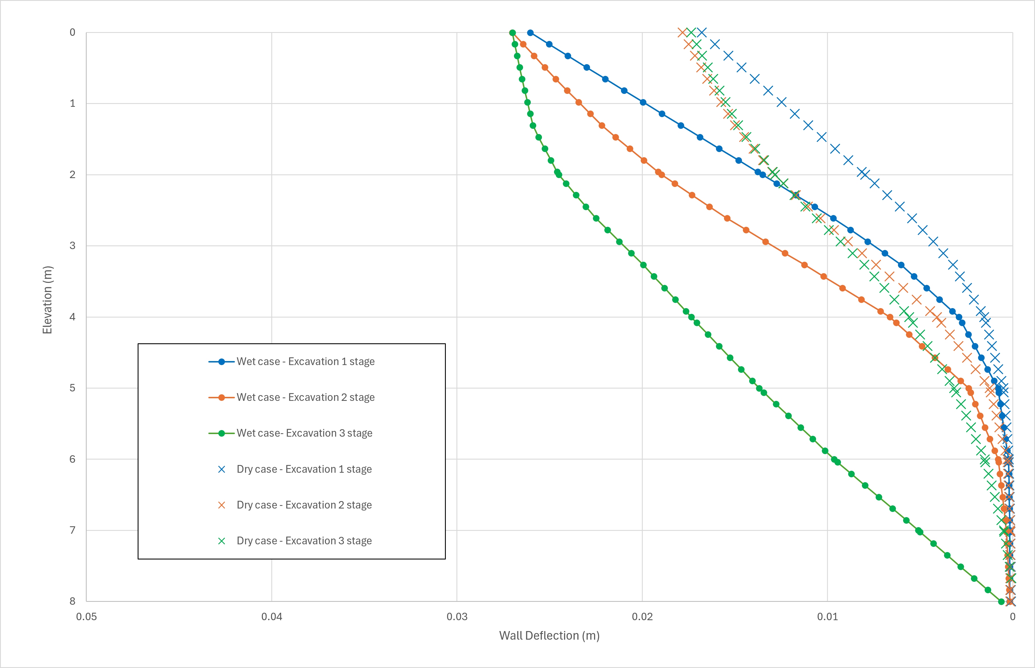
      Below are the graphs of the wet and dry cases exported to excel and combined:

      

13. Select all the SheetPile Wall entities from the Visibility Tree
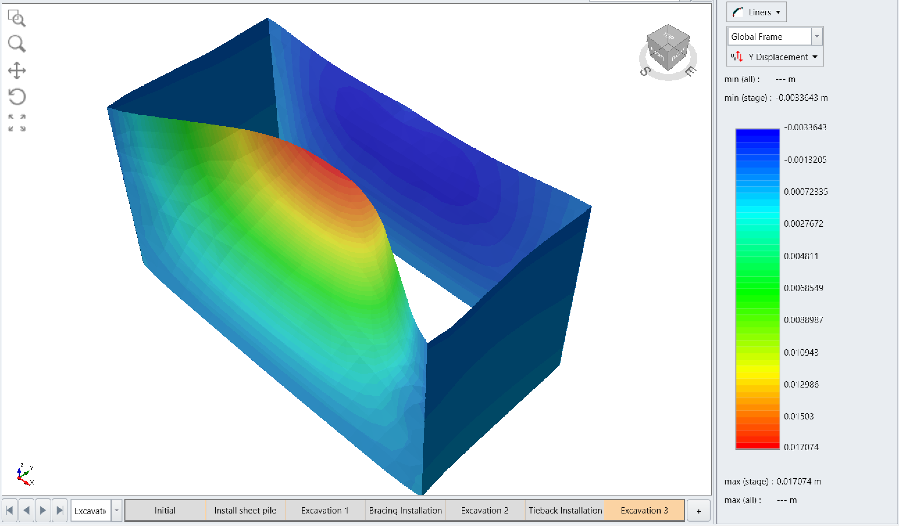
14. Select: Interpret > Deformed Configuration, which renders the exaggerated deformation pattern of the wall
15. Set the Legend to Liners and YDisplacement
16. Select the SheetPile Wall Deformation entities from the Visibility Tree
17. Right Click > Hide All But Selected Geometry

18. In the Properties Pane, set Scale Factor to 5 for each of the SheetPile Wall Deformation entities

    

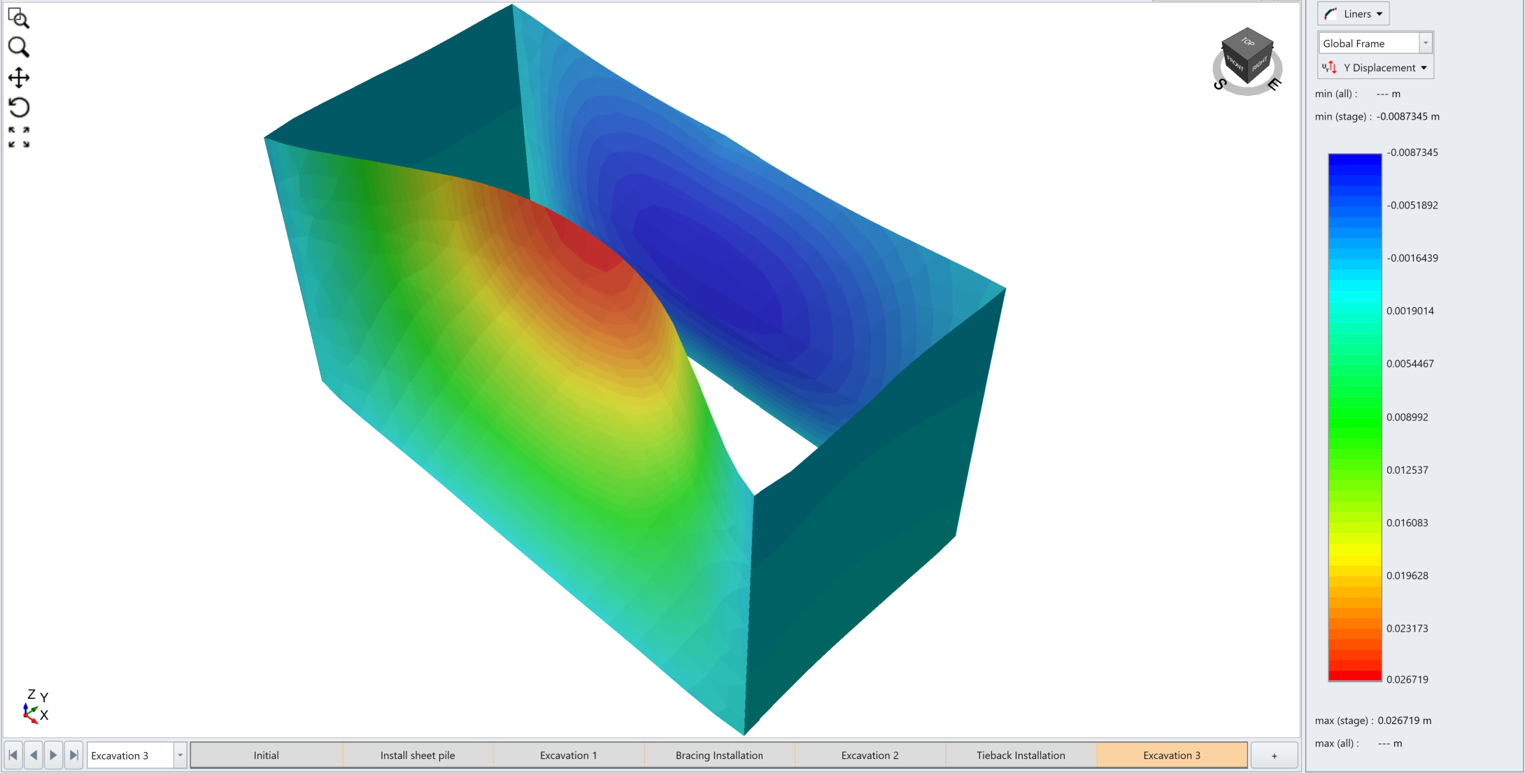
    Previous dry case:

    

This concludes the tutorial.