Liner Local Coordinates

1.0 Introduction

In this tutorial, we introduce the Liner local coordinates tool in RS3. This tool allows users to define local coordinate systems for groups of liners to better analyse the displacements, axial forces, shear forces and bending moments.

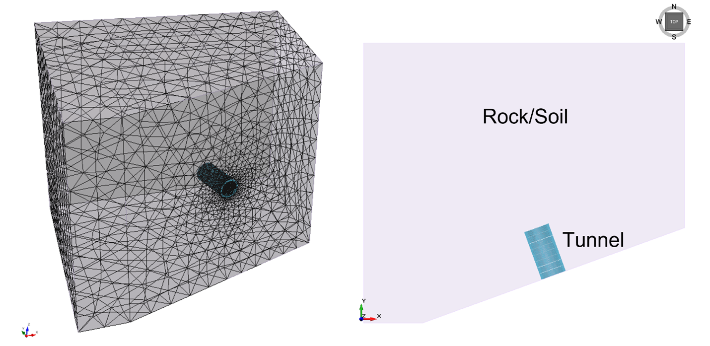
The model is based on the RS2 Tunnel Lining Design Tutorial-part 3. A circular tunnel of radius 4m is to be constructed in Schist at a depth of 550m. The tunnel axis is 20° counter-clockwise about the z-axis measured from the y-axis (trend angle of -20º). Taking the tunnel face an in-plane, the in-situ stress field has been measured with the major in-plane principal stress equal to 30 MPa, the minor in-plane principal stress equal to 15 MPa and the out-of-plane stress equal to 25 MPa. The major principal stress is on the horizontal plane and perpendicular to the tunnel axis. The minor principal stress is vertical. The strength of the Schist can be represented by the Generalized Hoek-Brown failure criterion with the uniaxial compressive strength of the intact rock equal to 50 MPa, the GSI equal to 50, and mi equal to 10. To compute the rock mass deformation modulus, the modulus ratio (MR) is assumed to be 400. The support is to be installed 2m from the tunnel face. The tunnel is excavated 2m per stage. In RS2, the tunnel wall deformation prior to support installation is estimated using the internal pressure reduction method. In RS3, we directly model the excavation and support installation staging to find the tunnel wall deformation. The RS3 model was created using the Tunnel Designer Tool.

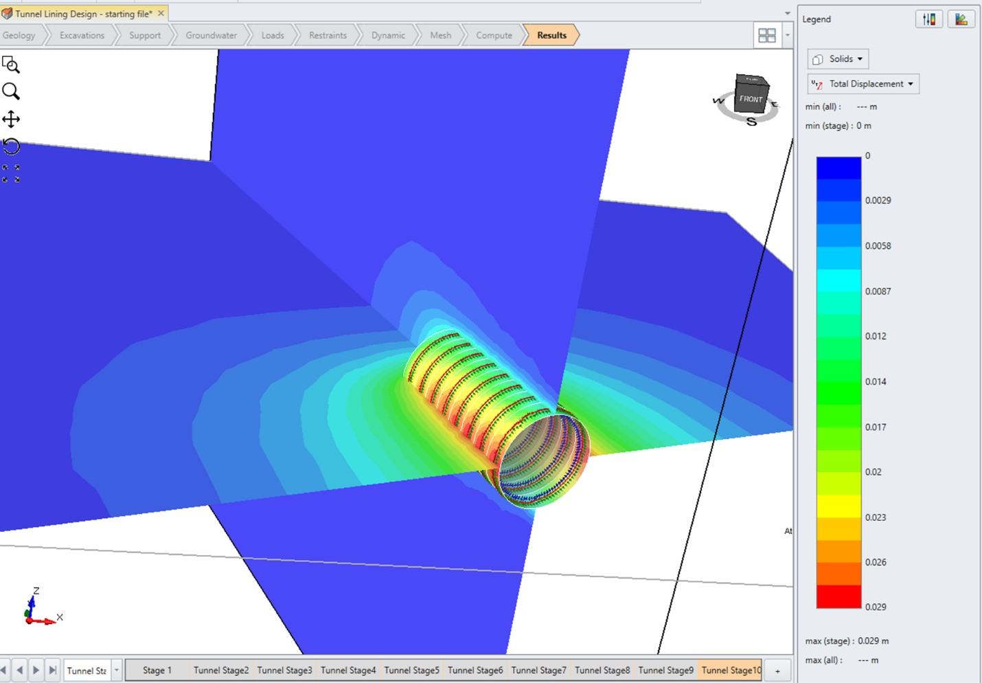
The image below shows the RS3 model of the rock/soil with tunnel excavation.

All tutorial files installed with RS3 can be accessed by selecting File > Recent > Tutorials folder from the RS3 main menu. The finished product of this tutorial can be found in the Tunnel Lining Design.rs3v3 file.

2.0 Starting the Model

1. Select File > Recent > Tutorials.
2. In the Tunnel Lining Design - starting file folder, open the Tunnel Lining Design - starting file.rs3v3.

All the project settings, material/support definitions, and tunnel sequencing are predefined in the starting file.

3.0 Defining the Liner Local Coordinates

The liner local coordinates can be defined under any tab.

1. We will select the Excavations workflow tab to better view the tunnel volumes.
2. Hide the Rock Mass external volume.
   
3. Select the tunnel side faces with Faces Selection mode active in the toolbar. Hold SHIFT when selecting a tunnel side face. This will quickly select all connected faces. Note that for the last tunnel volume, the tunnel end face may be selected as well when holding SHIFT. To deselect the tunnel end face, release SHIFT, hold CTRL and click on the tunnel end face. You may need to rotate your model to see the end face.
   
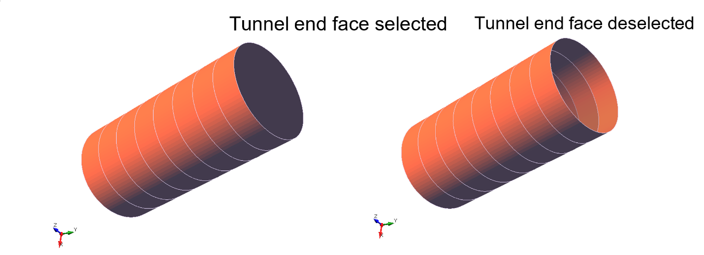
4. Select Support > Liners > Define Liner Local Coordinates for Tunnels
5. In the Define Liner Local Coordinates for Tunnels dialog under the Select Edge tab, we can input a vector manually or use the geometry to define the tunnel axis which will be the local y-axis. We can also choose to input trend and plunge angles in the Trend and Plunge tab. For this case, in the Select Edge Tab, select the pick edge tool (on the right side of the dialog) to use the geometry to define the tunnel axis. Now select any edge pointing in the tunnel axis direction and the vector coordinates will be automatically filled.
   
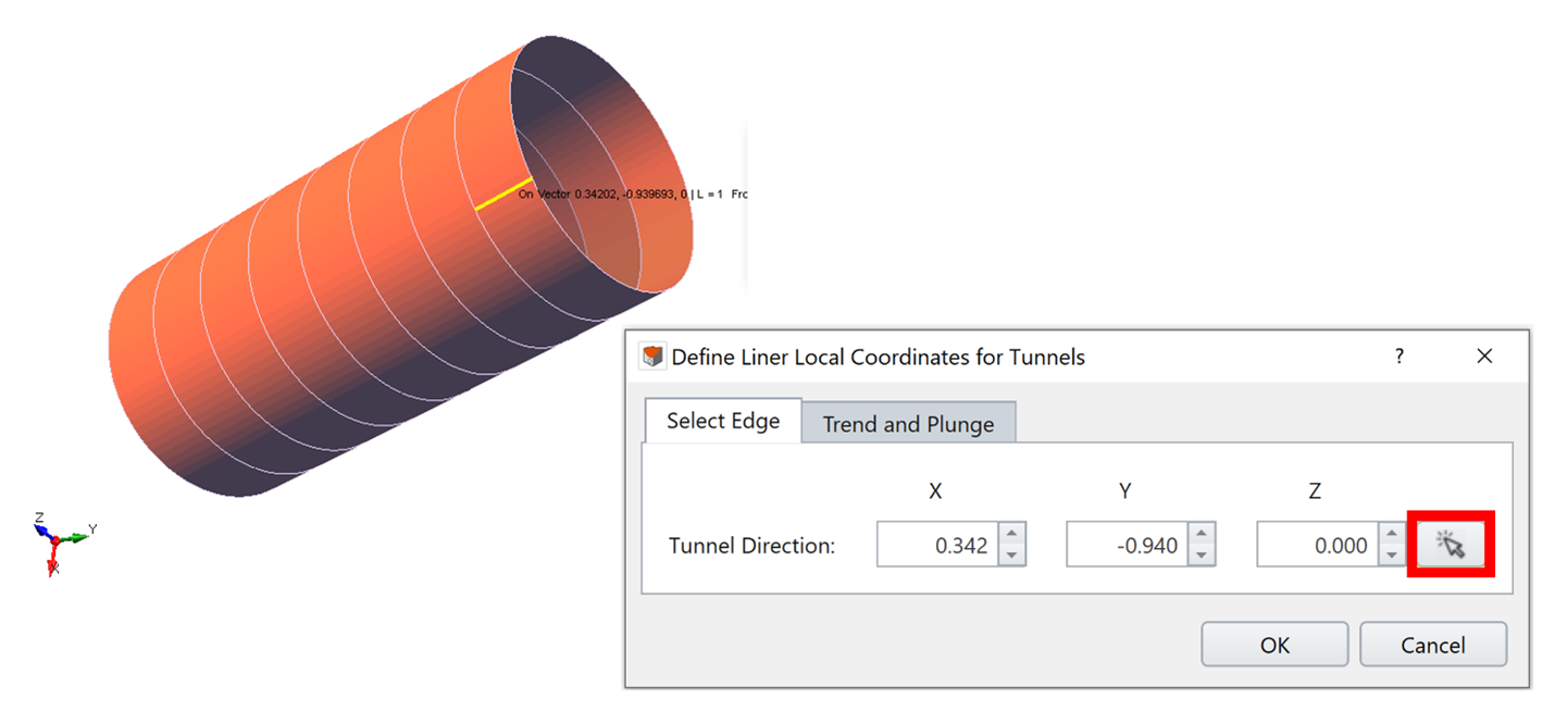
6. Click OK.

A new tunnel frame entity is created, which shows the local coordinate system for each side face of the tunnel. When defining a tunnel frame using the Define Local Coordinates for Tunnels option, it is important to select all faces that liner results will need to be converted to the frame's local coordinate system. Liner results that are not on a face defined in the tunnel frame are not guaranteed to be converted using the correct local coordinate system based on the liner's orientation at that point. There is also an option to manually define the local coordinate system using Support > Define Liner Local Coordinates which does not require the selection of faces. When using a frame defined in this manner, all liner results will be converted to the frame's local coordinate system.

4.0 Compute

1. Select the Compute workflow tab
2. From this tab, we can compute the results of our model. Before commencing the stress analysis computation, it is recommended to save the final model as a separate file so that you can access the original file anytime: File > Save As.
3. Select Compute > Compute

5.0 Results

1. Next, move to the Results workflow tab
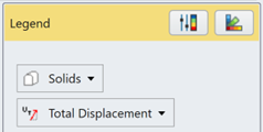
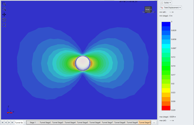
2. Select Tunnel Stage 10. To the right of the model, set the Legend to Solids and Total Displacement.

5.1 Tunnel Contour Results

1. Select Interpret > Show Exterior Contour
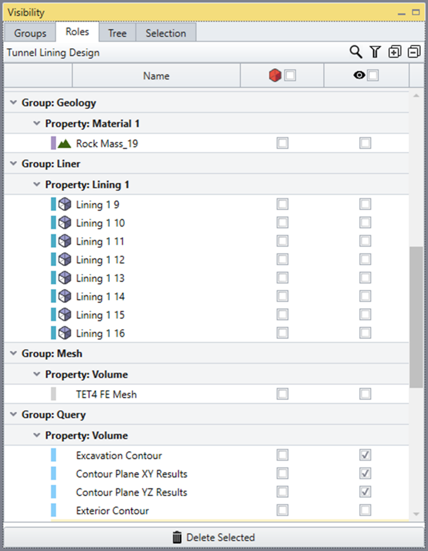
2. In the Visibility Pane, hide Excavation Contour, Contour Plane XY Results and Contour Plane YZ Results entities.
   
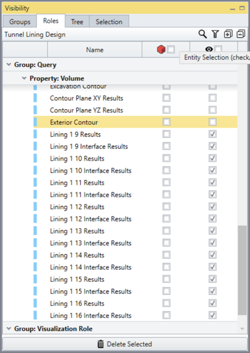
3. In the Visibility Pane under Roles, scroll down to Group: Query. Hide the Exterior Contours and show the following results: Excavation Contour, Contour Plane XY Results and Contour Plane YZ Results.
   

5.2 Liner Local Coordinates Results - Contour

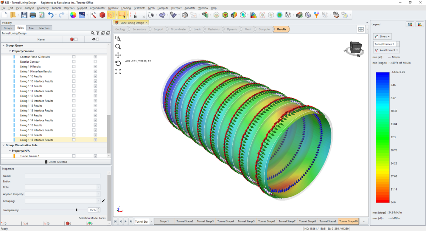
1. In the Legend, select Liners and Axial Force X.
2. In the Visibility Pane under Roles, scroll down to Group: Query again and ensure all Liner Results are visible.
   
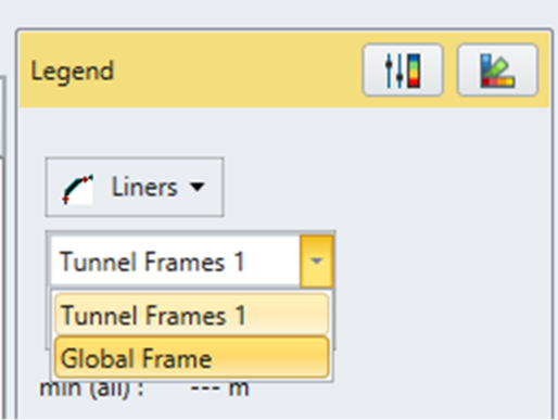
   Notice that in the Legend there is a drop-down menu below the Liners result type defining the liner coordinate frame used. The Global Frame refers to using the global coordinates as the liner coordinates for displaying results.
3. Change the frame to Tunnel Frames 1 which is the frame we defined earlier (as shown in the figure below). In this frame, the Axial Force X is the force along the hoop direction, tangent to the circumference of the tunnel.
   
   
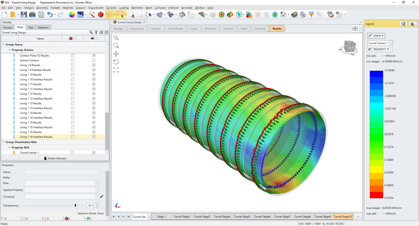
4. Set the Legend to Moment Y. This is the moment about the tunnel axis (local y-axis of Tunnel Frames 1).
   

Let's try plotting and exporting liner data in the current selected local liner coordinate frame.

5.3 Liner Local Coordinates Results - Query

A plane must be created to use the Add Liner Line Query at Intersection option, in the order to obtain liner query data around the tunnel wall at a specific location.

1. Select Geometry > 3D Primitive Geometry > Plane
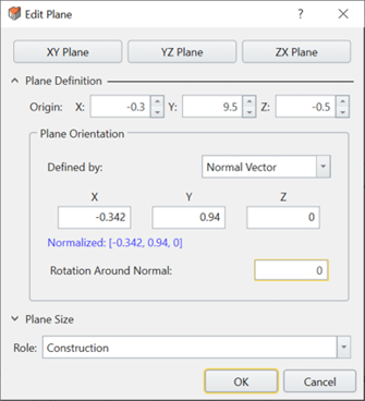
2. In the Edit Plane dialog, expand the Plane Definition section.
3. Set the Origin (X, Y, Z) to (-0.3, 9.5, -0.5).
4. Define the Plane Orientation by a Normal Vector of (-0.342, 0.94, 0).
5. Leave the Role as Construction and click OK. This creates a plane parallel to the circular tunnel face that fully cuts through the tunnel.
   
   
6. In the viewport and with Entity Selection mode active, hold CTRL and select the newly created Plane and the tunnel volume that it intersects called TNL 17: Region 0, Zone [4]_24. You can also select these entities in the Visibility Pane.
   
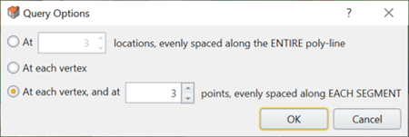
7. Select: Interpret > Queries > Add Liner Line Query at Intersection
8. Click OK in the Query Options dialog.
   
9. Hide the Plane and Tunnel Frames 1 entities. A liner line query has been created around the circumference of the tunnel. Ensure the Legend is set to Liners, Tunnel Frames 1 and Axial Force X.
   
10. To graph the Axial Force X along the liner line query, select the liner line query from the visibility tree.
11. In the Properties pane, click the Graph Data button. The graph will appear in a new Chart View tab.
    
    
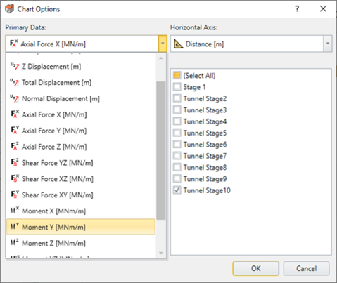
    In the Chart View tab, you can easily change plot data. Select the Change Plot Data button in the Chart Options pane. There are options to change the Primary Data, Horizontal Axis and plotted stages.
12. Try changing the Primary Data to Moment Y and select OK.
    
    
    
    A coarse mesh was used to improve computation speed as this tutorial focuses on showcasing the modelling process. A finer mesh would result in smoother plots.
    Let's export the data points.
13. Select Chart > Copy Data to Clipboard.

You can also select the Copy Data to Clipboard or right-click in the chart area and select Copy Data to Clipboard . The data are comma-separated values, which can be pasted and easily processed in Excel or any text editor. Below is the pasted data in Excel and converted to columns using their Text-to-Columns option that can delimit by commas.

This concludes the tutorial.