Scripting Tunnel Tutorial (Part 2)

1.0 Introduction

In the Scripting Tunnel Tutorial (Part 1), the model was created and computed using RS3 scripting. In this tutorial, the focus shifts to interpreting the computed results using scripting. RS3 provides a comprehensive set of result-querying tools that allow users to extract, process, and visualize analysis results programmatically.

The topics covered in this tutorial include:

Using the convergence status of the computed model to determine whether results should be queried
Querying solid and liner results within a defined region
Plotting and graphing the queried results

1.1 Tutorial Files

All tutorial files installed with RS3 can be accessed by selecting File > Recent > Tutorial Folder from the RS3 main menu. The tutorial files for this example can be found in the Scripting > Scripting Tunnel Tutorial (Part 2) subfolder, which is the final product of Scripting Tunnel Tutorial (Part 1).

This folder contains the Python script used for result extraction as well as the completed model generated in Scripting Tunnel Tutorial (Part 1).

This tutorial should begin after running the model. Without the computed model, result interpretation cannot proceed.

2.0 Open Model with Results

Open the RS3 program and start the scripting server by selecting Scripting > Manage Scripting Server > Choose an available port > Start Server. In this tutorial, port number 60064 is used.
Open the RocScript Editor through Scripting > RocScript Editor.
In the RocScript Editor, select File > Open Folder, and select folder C:\Users\Public\Documents\Rocscience\RS3 Examples\Tutorials\Scripting Tunnel Tutorial (Part 1). (Note: If you provided a custom location for examples when installing RS3, search the provided location instead.)
Navigate to the Explorer tab and select New file.
Name the new file Scripting_tutorial_result.py.

2.1 Import the Required Modules

The RS3Modeler module provides the primary interface for communicating with the RS3 application. Additional modules are imported to assist with geometry definition and result querying. Third-party libraries such as numpy and matplotlib are also used to process and visualize the results.

Import the required modules from the RS3 scripting API.

from rs3.RS3Modeler import RS3Modeler
from rs3.Geometry import Point, Cube
from rs3.results.ResultEnums import SolidsDataType, LinerResultTypes

Import third-party libraries for plotting and data processing.

import os
import matplotlib.pyplot as plt
import numpy as np

plt.style.use('ggplot')

Connect the script (client) to the RS3 Modeler application using the port number 60064.
```
port = 60064
modeler = RS3Modeler(port)
```
If you wish to launch the RS3 application automatically from the script, the function RS3Modeler.startApplication()can be used before creating the connection. When this function is called, you are not required to manually open the RS3 program or turn on the scripting server from RS3 modeler. However, ensure that the port number is unique. Using duplicated port numbers on the same computer may cause conflicts, which can prevent the script from connecting successfully.

Open the completed model generated from Scripting Tunnel Tutorial (Part 1) or you can use the finished product ready to be computed from the Scripting > Scripting Tunnel Tutorial (Part 2).

# Find the current file folder path
currentFileFolderPath = os.path.abspath("")

# Open the model
modelPath = rf"{currentFileFolderPath}\Scripting Tunnel Tutorial (Part 1) - Final.rs3v3"
model = modeler.openFile(modelPath)

The model in the tutorial folder is not computed.
You need the computed model in order to proceed further from this point. If you have the model computed from Part 1, you can use that file to proceed. However, make sure to redefine the currentFileFolderPath and the modelPath to properly reference that model. Alternatively, you can make a copy of this file inside the folder saved from Part 1.

3.0 Check Convergence

Understanding whether a model has converged at a given stage is important because convergence indicates that the numerical solution has stabilized and the results are reliable. If the solver fails to converge, it means the model's residual force/displacement did not fall below tolerance (default = 0.001) until the maximum number of iterations (default = 500) at some point of load steps. In such case, the computed results from that stage may not be reliable, so users should treat them with caution or exclude them from further analysis.

The convergence summary is particularly useful when automating result extraction. When running multiple models or stages in scripts, it is advisable to check the convergence status of the model. The method, `model.Compute.readConvergenceStatus()`, outputs a tuple of a Boolean to represent the success of model computation, a string of error message if unsuccessful, and a list of convergence status per stage. With the returned information, you can programmatically filter out failed models or non-converged stages from mechanical analyses or post-result processing.

Extract the convergence status of the model.

If the model did not finish computing, success will be False, and an error message will be returned in errorMessage. If the computation completed successfully, users can proceed to check the convergence status of each stage using convergenceStatus.

success, errorMessage, convergenceStatus = model.Compute.readConvergenceStatus()\
print(f"Success: {success}")
print(f"Error Message: {errorMessage if errorMessage else "No error message."}")
print(f"convergenceStatus: {convergenceStatus}")

Success: True
Error Message: No error message.
convergenceStatus: <rs3.Compute.StageSRFValueConvergenceStatus object at 0x000001C8E7A597F0>

ConvergenceStatus contains both StagesConvergence results and SrfValuesConvergence results. Since this model only performs stress analysis, we will focus on checking the convergence results for each stage.
```
print(convergenceStatus.StagesConvergence)
```
```
[(1, True), (2, True), (3, True), (4, True), (5, True), (6, True), (7, True), (8, True), (9, True), (10, True)]
```

4.0 Query Solids Results

All solid results can be queried directly at either the node level or the element level. This provides users with additional flexibility to work with the raw result data, enabling more advanced data processing and analysis. For example, users can perform custom calculations such as averaging values, filtering results, or applying their own post-processing methods.

Scripting also allows users to specify which result data types should be loaded for analysis. Since different workflows may require different types of results, this capability allows users to load only the data relevant to their task. As a result, the results loading process can be more efficient, particularly when working with large models or when only a subset of results is required.

# first, get the results object from the model
results = model.Results

4.1 Load Solid Results

Once the stage convergence status is known, we first check whether the stage converged. If the stage converged, query the Z-displacement results at the ground surface to measure the settlement due to excavation. The querying solid data type is used here to reduce the data loading time during result extraction.

queryStageNumbers = list(range(3, 9))
solidDataTypes = [SolidsDataType.DISPLACEMENT_Z]

# Check convergence status for all query stages
allConverged = all(convergenceStatus.StagesConvergence[stage-1][1] for stage in queryStageNumbers)

# If all stages converged, get mesh results. Otherwise, do not query results.
if allConverged:
 solidResults = results.getMeshResults(stageNumber=queryStageNumbers, requiredDataTypes=solidDataTypes)
else:
 print("Not all query stages are converged. Results will not be queried.")

4.2 Query Surface Vertical Displacement

In this section, the vertical displacement at the ground surface is extracted and plotted to observe the settlement profile along the tunnel alignment.

Define a query region to capture the nodes near the ground surface above the tunnel.
```
surfaceSolidQueryRegion = Cube(Point(-0.2, -1.0, 799.5), Point(0.2, 40, 798.5))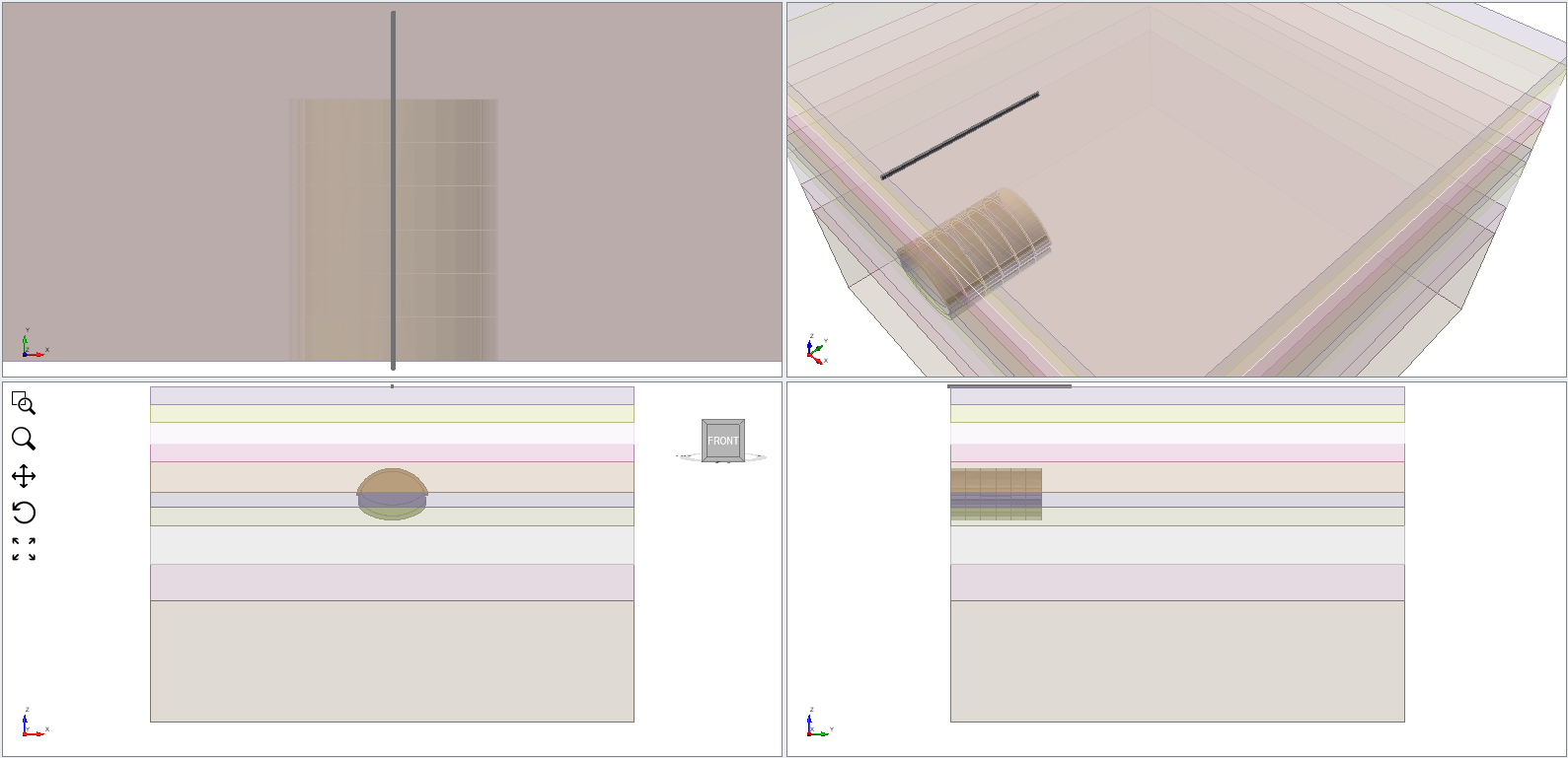
```
Note: The 'Cube' class method in scripting does not actually create a geometry entity. The figure is simply to aid the visualization of the 'surfaceSolidQueryRegion' object

Query solid nodal results per stage and save the results to surfaceSolidResults.

# Create an empty list to save solid results
surfaceSolidResults = []

# This for-loop loops through solid result of each stage loaded at the last step
for surfaceSolidResultsPerStage in solidResults:
 # Get the node result objects in the given region of each stage
 surfaceStagedSolidResults = surfaceSolidResultsPerStage.getMeshNodeResults(region=surfaceSolidQueryRegion)
 # Save the result in the list
 surfaceSolidResults.append(surfaceStagedSolidResults)

The returned nodes are ordered based on their node IDs. To produce a clearer plot, the nodes will be reordered according to their Y-coordinates.

# Use first queried stage (Stage 2) to get node order
firstStageNodes = surfaceSolidResults[0]

# Sort indices by YCoordinate
sortedY, sortedIndices = zip(*sorted(
 ((node.YCoordinate, idx) for idx, node in enumerate(firstStageNodes)),
 key=lambda x: x[0]
))
sortedY = list(sortedY)
sortedIndices = list(sortedIndices)

Retrieve the vertical displacement of all nodes at the queried stages.

# Create an empty list for saving node Z displacement data of all stages
nodeZDisplacementQueriedStages = []

# set the grouting starting stage as a variable
groutingStartingStage = 2

# Only query from stage 2 to stage 22, so the index of stages can be obtained here
for queriedStage in surfaceSolidResults:
 # Create an empty list to save node Z displacement result per stage
 nodeZDisplacementPerStage = []
 for node in queriedStage:
 # Get the solid Z displacement results which is loaded previously
 nodeZDisplacement = node.getResult(SolidsDataType.DISPLACEMENT_Z)
 # Save the node results of this this stage
 nodeZDisplacementPerStage.append(nodeZDisplacement)
 # Save the node Z displacement results of all stages
 nodeZDisplacementQueriedStages.append(nodeZDisplacementPerStage)

Get the stage names of the queried stages.

stageNames = [model.ProjectSettings.Stages.getName(stageNumber) for stageNumber in queryStageNumbers]

Plot the surface settlement profile (Vertical Displacement vs. Distance).

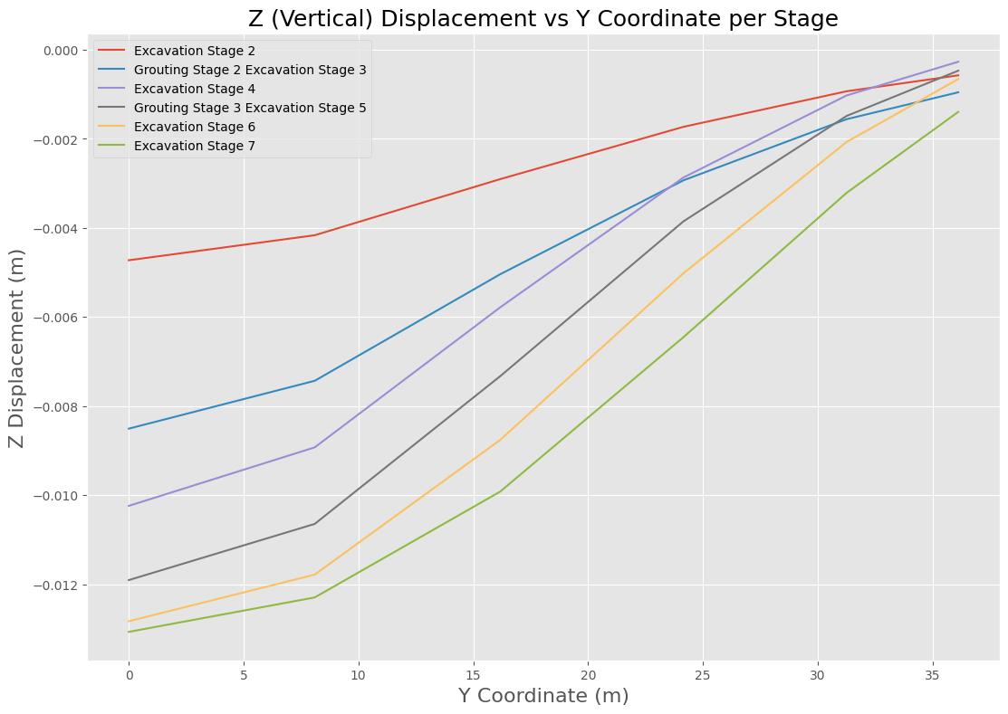
# Convert total displacement data as a numpy array
nodeZDisplacementQueriedStagesArray = np.array(nodeZDisplacementQueriedStages)

# Create an empty figure with the figure size
plt.figure(figsize=(13, 9))

# Get the size of the nodeZDisplacementAllStagesArray
for stageIndex in range(nodeZDisplacementQueriedStagesArray.shape[0]):
 # Reorder displacement according to sorted Y
 sortedDisplacement = nodeZDisplacementQueriedStagesArray[stageIndex, sortedIndices]
 # Plot
 plt.plot(sortedY, sortedDisplacement, label=f"Stage {queryStageNumbers[stageIndex]}")

# Set the X-axis label
plt.xlabel("Y Coordinate (m)", fontsize=16)
# Set the Y-axis label
plt.ylabel("Z Displacement (m)", fontsize = 16)
# Set the title of the plot
plt.title("Z (Vertical) Displacement vs Y Coordinate per Stage", fontsize=18)
# Create a legend and set the legend of the plot
plt.legend(stageNames)
# Turn on the plot grids
plt.grid(True)

# (Optional) You may save the plot for the report.
plt.savefig("Vertical Displacement vs. Y Coordinates.png", dpi=300, bbox_inches="tight")

# Show the plot
plt.show()

The resulting plot illustrates the evolution of surface settlement during the excavation process.

5.0 Query Liner Results

Liner results such as axial force, shear force, and bending moment can also be extracted using scripting. In this section, the bending moment distribution along the tunnel liner is evaluated.

Load liner results from the final stage.

lastStageNumber = 10
if convergenceStatus.StagesConvergence[lastStageNumber-1][1]:
 linerResults_st22 = results.getCompositeLinerResults(stageNumber=[lastStageNumber])[0]
else:
 print("Stage {lastStageNumber} didn't converge. Results will not be extracted.")

Set the coordinate system for the liner results to the predefined frame, "Tunnel Frame 1". The tunnel frame defines the local X-axis to follow the circumference of the tunnel and Y-axis to align the tunnel path. See more information about Liner Local Coordinate here.
```
localCoordinateSystemName = "Tunnel Frames 1"
linerResults_st22.setCoordinateSystem(localCoordinateSystemName)
```
Define a query region around the tunnel liner.
```
linerQueryRegion = Cube(Point(-12, 12.25, 754), Point(12, 12.75, 771.5))
linerElementResults_st22 = linerResults_st22.getLinerElementResults(region=linerQueryRegion)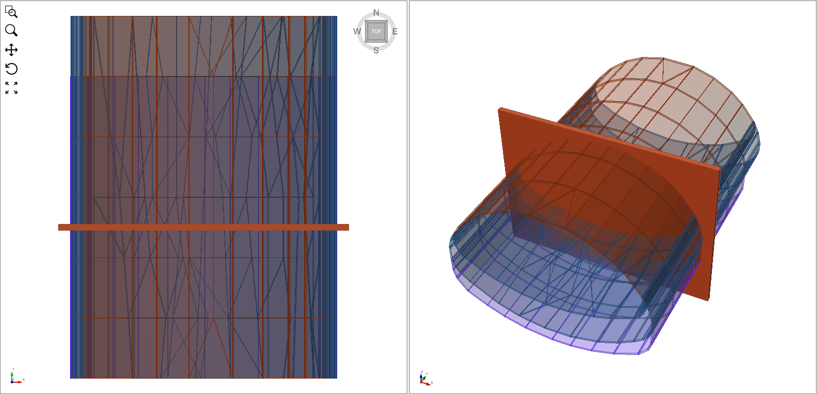
```
Note: The 'Cube' class method in scripting does not actually create a geometry entity. The figure is simply to aid the visualization of the 'linerQueryRegion' object

Retrieve the moment about the Y-axis (My) for each liner node and store the values in a list. If there are multiple moment values at the same node, the average moment will be calculated.

from collections import defaultdict

# Initialize dictionaries to collect sums and counts
moment_sum = defaultdict(float)
count = defaultdict(int)

# Loop through all element results
for element in linerElementResults_st22:
 node_ids = element.AttachedNodeIDs
 moment_values = element.getResults(LinerResultTypes.MOMENT_YY)
 
 for nid, moment in zip(node_ids, moment_values):
 moment_sum[nid] += moment
 count[nid] += 1
 
# Compute averages
node_moment_avg = {nid: moment_sum[nid]/count[nid] for nid in moment_sum}

Query the location of all queried nodes.

nodeInfo = results.queryNodeInfoFromLiners(lastStageNumber)
node_location = {}

for node in nodeInfo:
 node_location[node.nodeID] = node.location

Clean up the duplicated nodes, since the moment is the averaged moment.

# Use only nodes present in the averaged results
node_ids = list(node_moment_avg.keys())
x = np.array([node_location[nid][0] for nid in node_ids])
z = np.array([node_location[nid][2] for nid in node_ids])
moment = np.array([node_moment_avg[nid] for nid in node_ids])

# Remove duplicated coordinate points
coords = np.column_stack((x, z))
_, unique_idx = np.unique(coords, axis=0, return_index=True)

# Keep the first occurrence of each coordinate
unique_idx = np.sort(unique_idx)

x = x[unique_idx]
z = z[unique_idx]
moment = moment[unique_idx]

Sort the order of nodes.

# Compute tunnel center
cx = np.mean(x)
cz = np.mean(z)
print(f"The center of tunnel is ({cx}, {cz}).")

# Sort nodes counterclockwise
angles = np.arctan2(z - cz, x - cx)
# Sort the index of nodes based on the angle
sort_idx = np.argsort(angles)

# Rearrange the arrays using the sorted indices.
x = x[sort_idx]
z = z[sort_idx]
moment = moment[sort_idx]

Calculate the scaled moment as the magnitude of moment.

# Compute the gradient of x and z along the ordered nodes.
# These approximate the local tangent direction of the tunnel boundary.
dx = np.gradient(x)
dz = np.gradient(z)

# Compute the length (magnitude) of the tangent vector at each node.
# This is used to normalize the direction vectors.
length = np.sqrt(dx**2 + dz**2)

# normal x
nx = -dz / length
# normal z
nz = dx / length

# Scale factors for visualization
moment_scale = 0.003

# Offset for moment and axial diagrams
x_m = x + moment * moment_scale * nx
z_m = z + moment * moment_scale * nz

Plot the liner moment diagram.

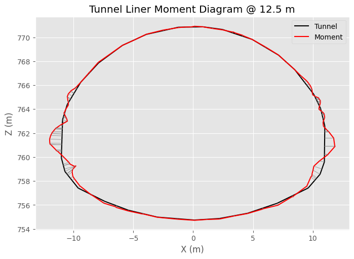
# Close the tunnel geometry
x_closed = np.append(x, x[0])
z_closed = np.append(z, z[0])

# Close the moment diagram
x_m_closed = np.append(x_m, x_m[0])
z_m_closed = np.append(z_m, z_m[0])

# Set the figure size
plt.figure(figsize=(8, 8))
# Plot the tunnel outline
plt.plot(x_closed, z_closed, 'k', label="Tunnel")
# Plot the moment diagram
plt.plot(x_m_closed, z_m_closed, 'r', label="Moment") 

# Draw lines showing magnitude
for i in range(len(x)):
 plt.plot([x[i], x_m[i]], [z[i], z_m[i]], 'gray', linewidth=0.5)

# Make sure the x and y axes are in the equal scaling
plt.gca().set_aspect('equal')
# Turn on the grid
plt.grid(True)
# Turn on the legend
plt.legend()
# Define the x and y labels of the plot
plt.xlabel("X (m)")
plt.ylabel("Z (m)")
# Set the plot title
plt.title("Tunnel Liner Moment Diagram @ 12.5 m")

# (Optional) You may save the plot for the report.
plt.savefig("Tunnel Liner Moment Diagram @ 12.5 m.png", dpi=300, bbox_inches="tight")

# Show the plot
plt.show()

The plot shows the scaled moment distribution around the tunnel perimeter

6.0 Close the Program

Since the script only queries results and does not modify the model, the project can be closed without saving.

model.close(False)

After all result extraction tasks are completed, the RS3 application can also be closed.

modeler.closeProgram(False)

This concludes the Scripting Tunnel Tutorial (Part 2).

All User Guides

Search Results