Dynamic Analysis of Foundation

1.0 Introduction

This tutorial will demonstrate some of the dynamic analysis features of RS3. Here we simulate a foundation experiencing cyclic machine loading

All tutorial files installed with RS3 can be accessed by selecting File > Recent > Tutorials folder from the RS3 main menu. The finished product of this tutorial can be found in the Dynamic Analysis of Foundation.rs3v3 file. The starting file can be found in Dynamic Analysis of Foundation - starting file.rs3v3 file.

2.0 Starting the Model

1. Select File > Recent > Tutorials Folder in the menu.
2. In the folder Dynamic Analysis of Foundation - starting file, open the starting file Dynamic Analysis of Foundation - starting file.rs3v3.

All the project settings and material definitions are predefined in the starting file. Read through these two sections to make sure the inputs in the model are consistent with this tutorial.

1. Select: Analysis > Project Settings
   
2. In Units tab, set Units = Metric, stress as kPa.
   
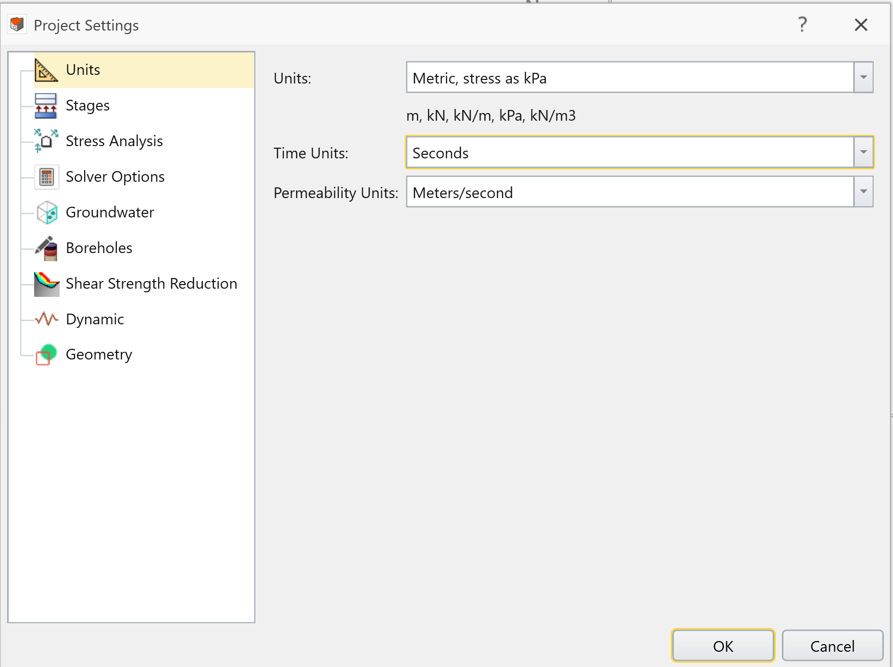
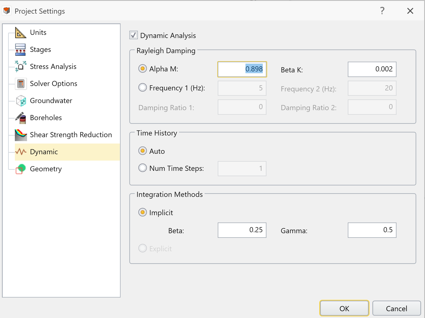
3. Next, select the Dynamic tab.
4. Enter following properties:
   
   1. Tick the Dynamic Analysis checkbox
   2. Alpha M = 0.898
      
   3. Beta K = 0.002
      
   4. Time History = Auto
      



5. Select the Stages tab and enter the following properties:
   1. Number of Stages = 5

#	Name	Time (Seconds)	Dynamic
1	Stage 1	0
2	Stage 2	0.7	YES
3	Stage 3	0.73	YES
4	Stage 4	0.75	YES
5	Stage 5	0.5	YES



6. Do not change any other settings.
   
7. Click OK to close the dialog.

3.0 Defining the Materials

Under the Geology or Excavations workflow tab you can assign the materials and properties of the model through materials setting.

The starting file should already have these values provided for the user. Just make sure the values in these tutorials are consistent with the model.

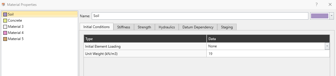
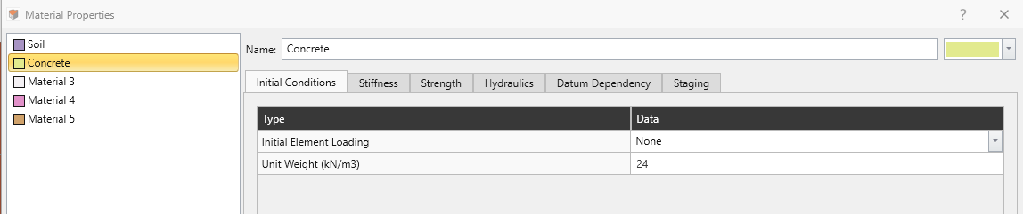
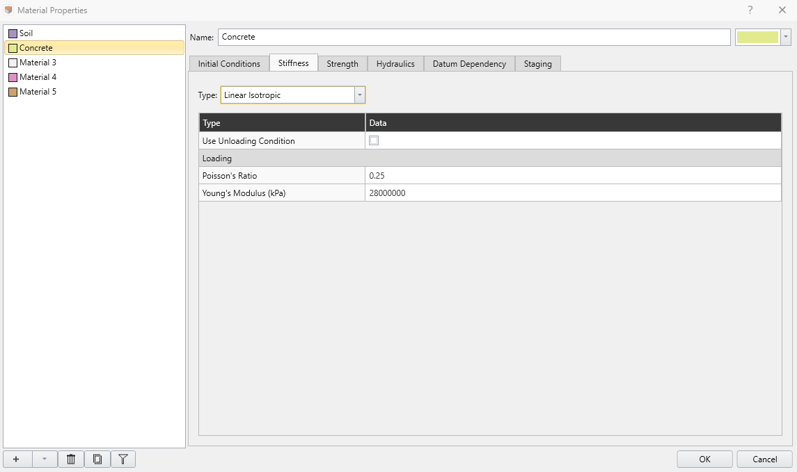
1. Select: Materials > Define Materials.

Soil [Initial Conditions]:

Concrete [Initial Conditions]:

Soil [Stiffness]:

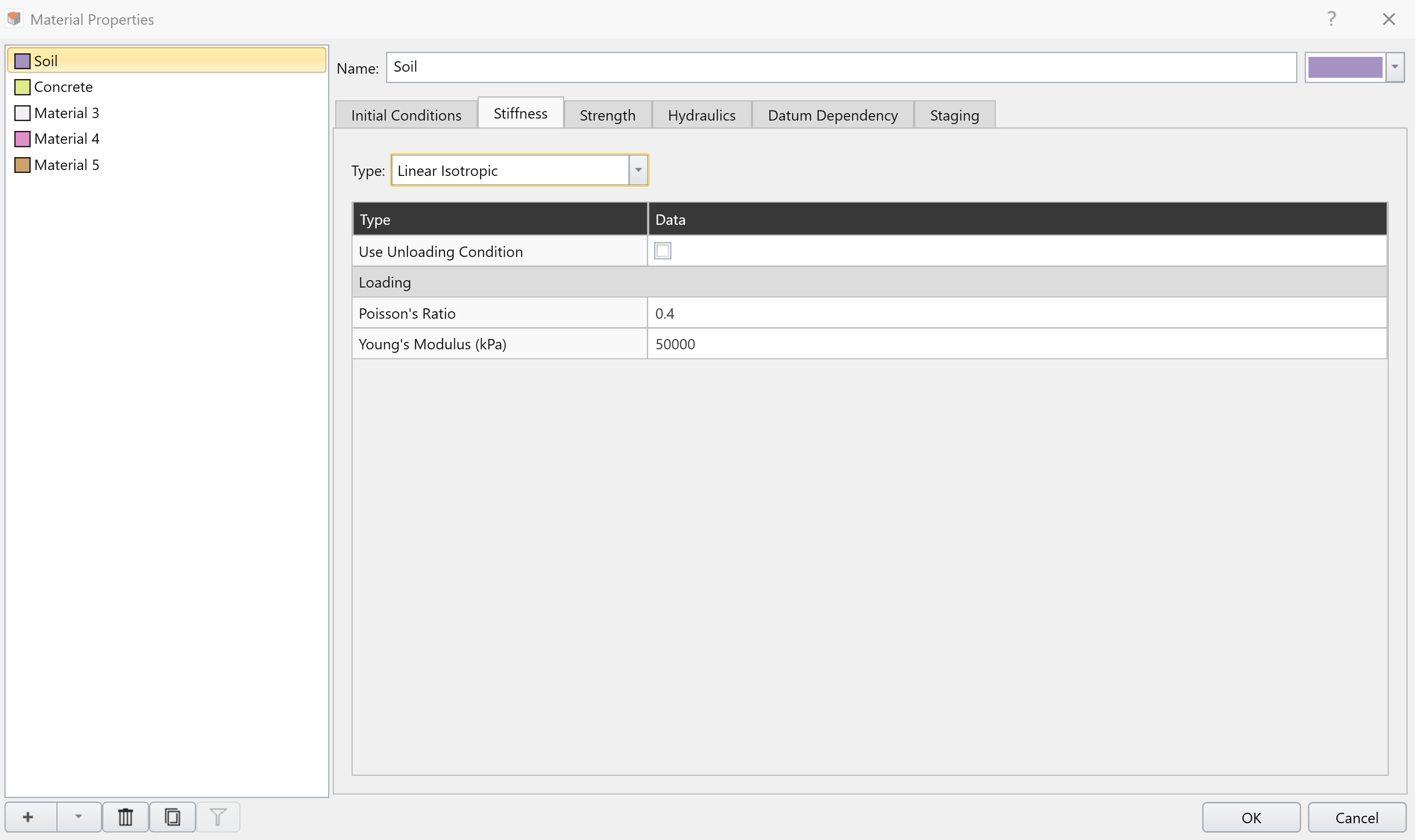
Concrete [Stiffness]:

4.0 Creating the Geometry

4.1 CREATING THE GROUND

In order to create the ground, we will generate a rectangular prism.

1. Select: Geometry > 3D Primitive Geometry > Box
2. A Create Box dialog will open. Enter First Corner (x, y, z) = (0, 0, 0), Second Corner (x, y, z) = (140, 70, 70).
   
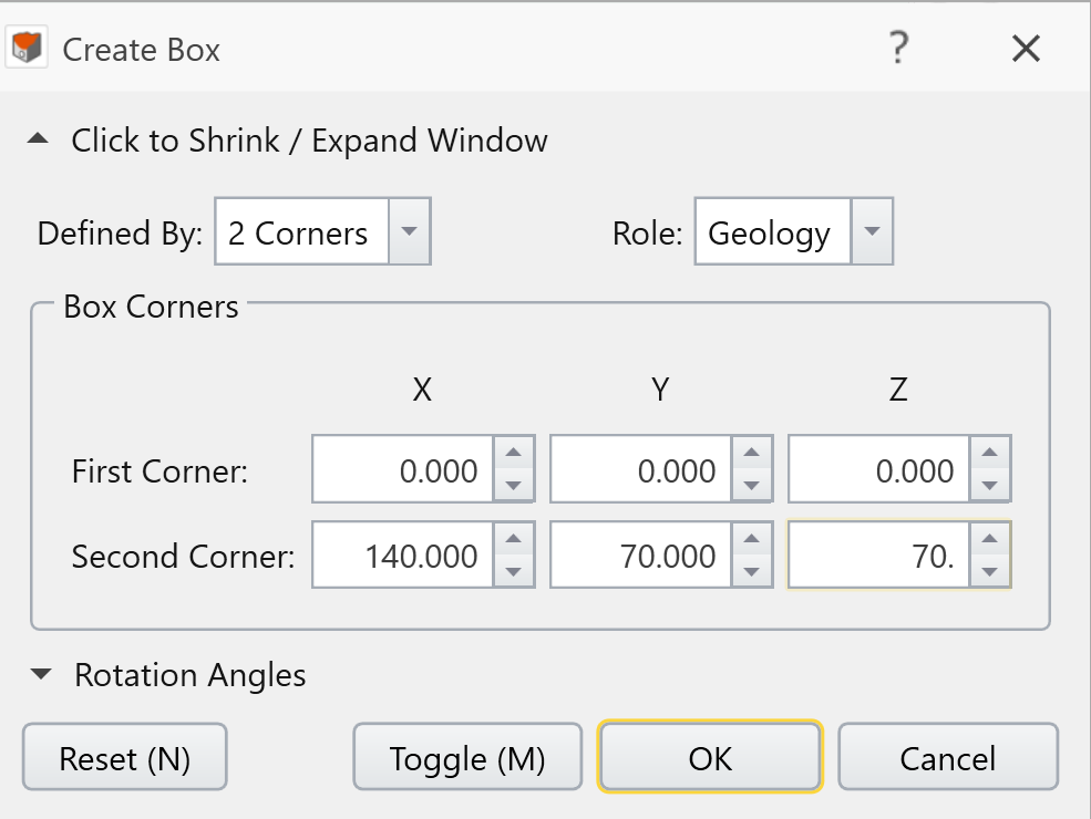
3. Click OK.

To create a foundation with 0.4 m thickness and 8 m x 8 m cross section dimension, we will generate another rectangular prism with the geometry as defined in the following.

4. Select: Geometry > 3D Primitive Geometry > Box
5. Enter First Corner (x, y, z) = (66, 31, 69), Second Corner (x, y, z) = (74, 39, 70.4).
   
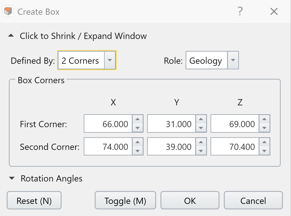
6. Click OK.

4.2 PREPPING THE EXTERNAL BOUNDARIES

To capture the extents of the model as the external boundary, the foundation must be merged with the ground. But as they are made of different materials, we also need to create a cutting plane between the merged bodies.

1. Select both bodies (Box and Box 2) in the Visibility pane.
   
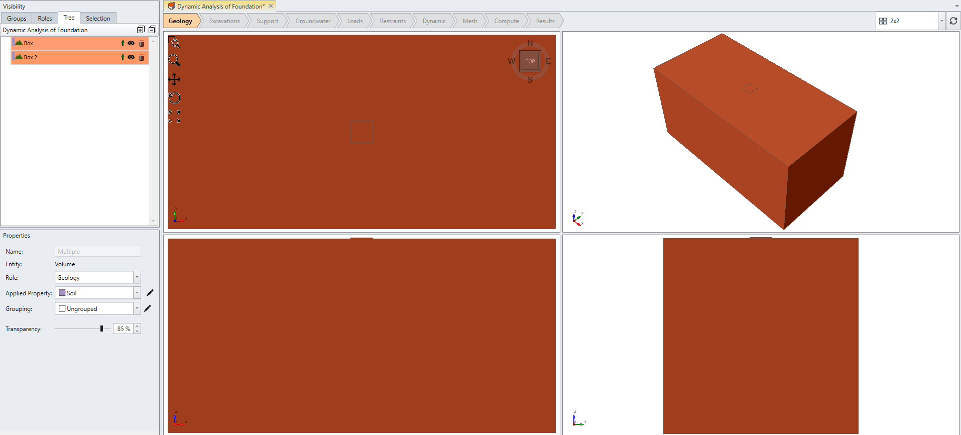
2. Select: Geometry > 3D Boolean > Union
3. Click OK. Then, select the “union w/ Box” body in the Visibility pane.
4. Select: Geometry > Set as External
   

To define the cutting plane:

5. Select: Geometry > 3D Primitive Geometry > Plane
6. Select XY Plane. Under Plane Definition, set Origin (x, y, z) = (70, 35, 70).
   
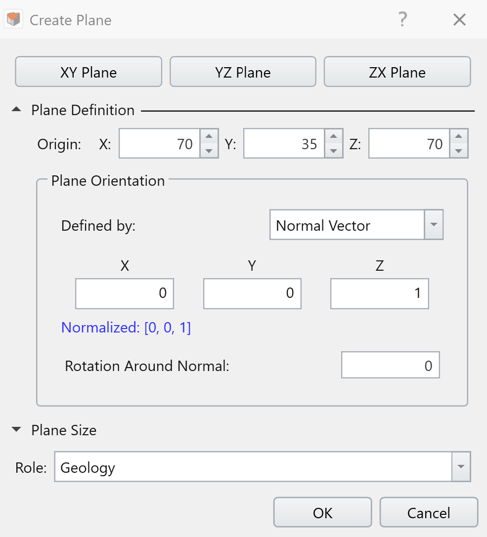
7. Click OK.

4.3 DIVIDING THE MODEL

1. Select: Geometry > 3D Boolean > Divide All Geometry . Click OK with default quality.
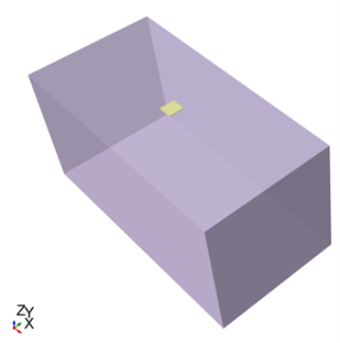
2. Ensure all bodies have Role = Geology, (can do so by seeing if all bodies have the geology icon in the visibility pane). Change the foundation body to Concrete by selecting “union w/Box_2” in the visibility pane, and in the properties pane change Applied Property = Concrete. After doing so, the model should look like:

5.0 Setting Boundary Conditions

1. Move to the Restraints workflow tab to assign restraints to the external boundary of the model.

As dynamic analysis is computed for Stage 2 - Stage 5, the Dynamic Boundary Condition is assigned for those stages and the displacement restraints should be applied for solely Stage 1. Since Initial Element Loading is set to be "None" for both materials, any deformation is prevented in Stage 1; however, it is good practice to always have appropriate boundary conditions assigned to the model.

In this case, we need to use Staging options to specify the stage at which the displacements will be installed and the stage at which the displacements will be removed.

2. For custom restrain definition, select the following faces in the model (using Face Selection in the toolbar):
   
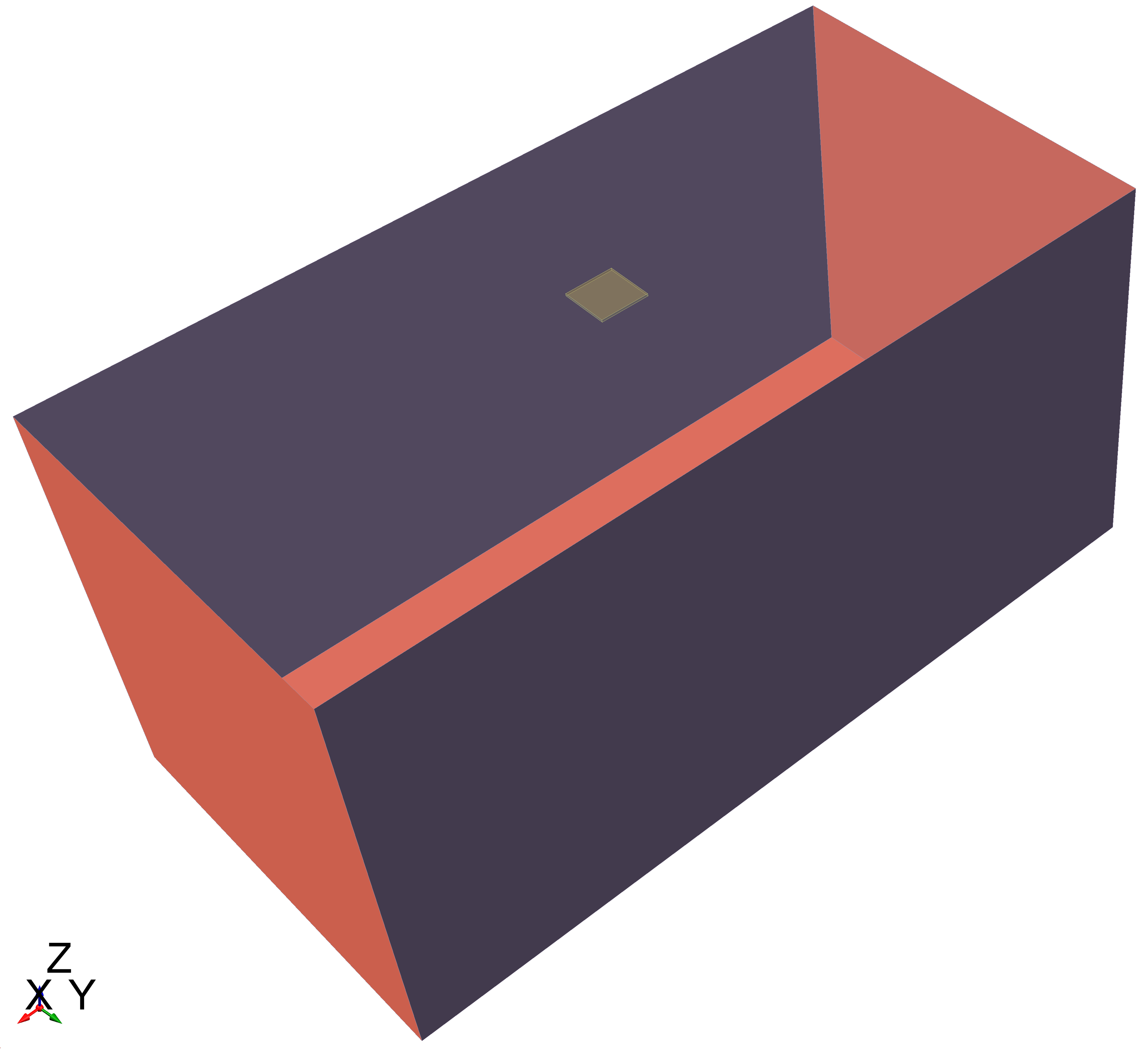
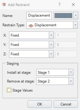
3. Select: Restraints > Add Restraints/Displacements > Displacements
4. Apply the Settings as shown below:
   1. Make sure it is installed at Stage 1 and removed at Stage 2

If you select the Dynamic Face in the visibility pane, you will notice the bar above Stage 1 tab is in grey (indicating that the restraint is applied), and the bars above Stage 2-5 are in black (indicating that the restraint is removed).

6. Setting Dynamic Condition

6.1 LOADING THE MODEL

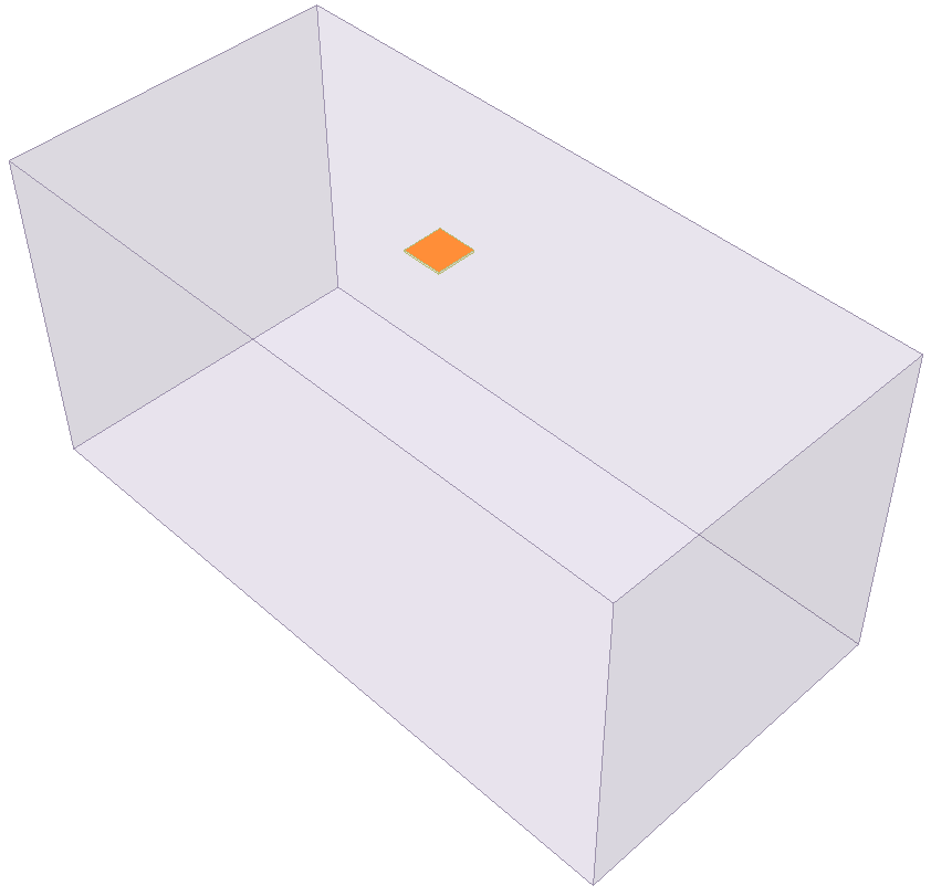
1. Select the top concrete surface
   
2. Select: Dynamic > Add Dynamic Loads
3. Select the pencil edit icon beside the Dynamic Property dropdown to edit the loading.
   
   
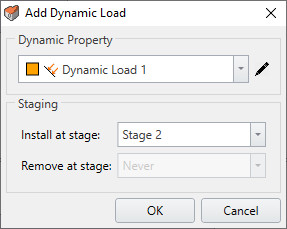
4. Set Name = Dynamic Load, Type = Force, Custom = Active, X: = Active, then select [Define…] next to X.

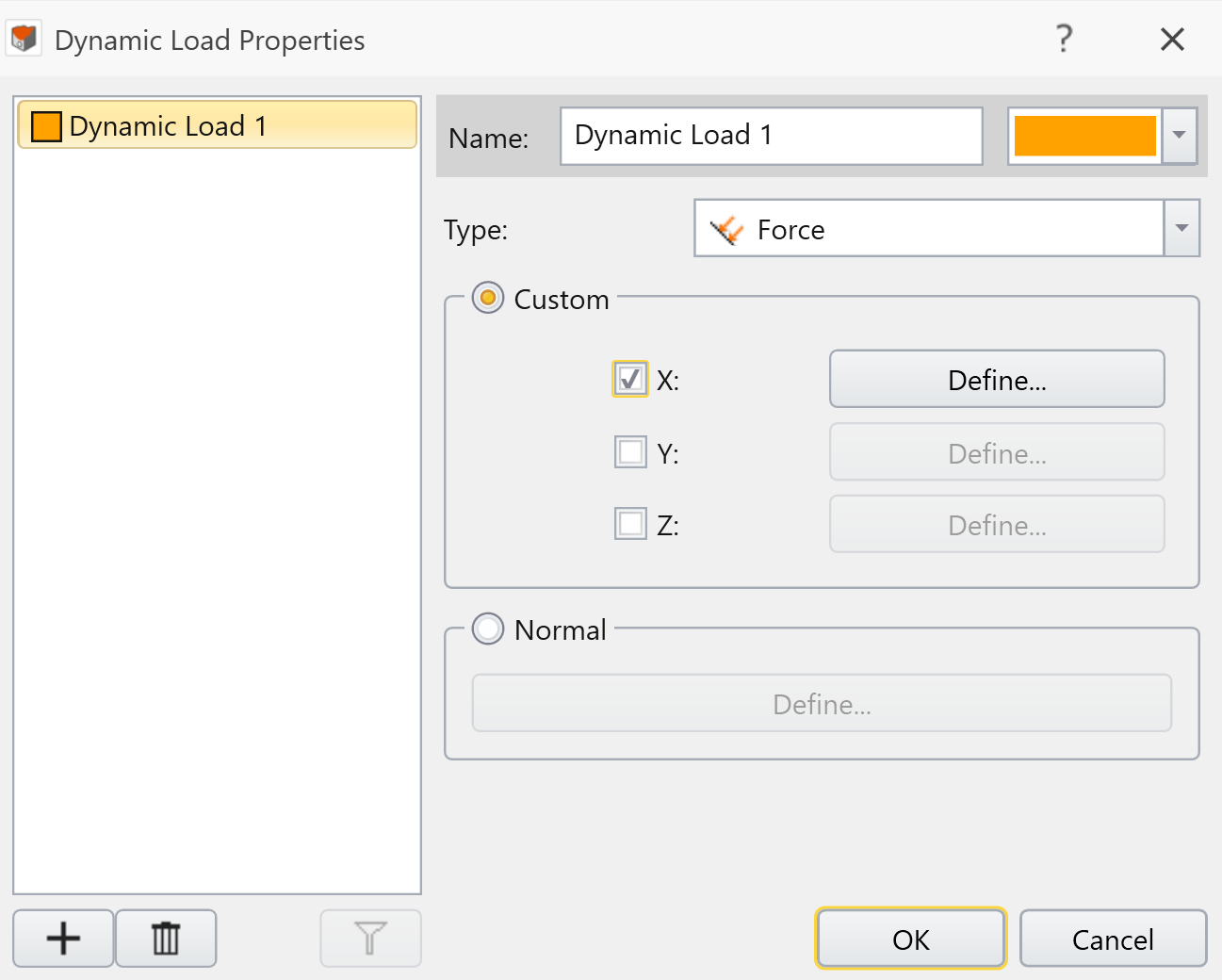
A new Define Dynamic Load Force By Time dialog will open.The data can be found in the tutorial folder.

5. Open the machine_load.txt file from Dynamic Analysis of Foundation - starting file folder. Copy the first column data and paste to the dialog as Time (seconds). Copy the second column data and paste to the dialog as Force (KN/m/m).
6. The Force-Time graph based on the input data can be loaded by clicking Show Chart icon



7. When all values have been copied over, click OK to confirm and close all dialogs.

You should now notice that as you flip between Stage 1 and 2, the loading will toggle on and off on 3D modeler view, as the load begins to be applied at Stage 2 (the first dynamic stage). If you select the Dynamic Load 1 Face in the visibility pane, you will notice the bar above Stage 1 tab is in white (indicating no load), and the bars above Stage 2-5 are in orange (indicating dynamic load is applied).

6.2 ADDING BOUNDARY CONDITION

1. Select all four side faces, and the bottom face of the ground (five faces total).
   
2. Select: Dynamic > Add Dynamic Boundary Conditions
3. Select the pencil edit icon beside the Dynamic Property dropdown to edit the boundary condition. A Dynamic BC Properties dialog should appear, set Type = Absorb, then click OK for Dynamic BC Properties dialog and click OK again for Add Dynamic BC dialog.
   

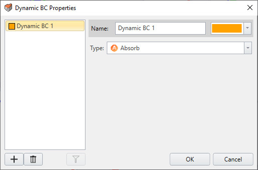
You should now notice that as you flip between Stage 1 and 2, the Absorb BC will toggle on and off, as the load begins to be applied at Stage 2 (the first dynamic stage).

6.3 ADDING A DYNAMIC QUERY LINE

1. Select: Dynamic > Add Time Query
2. In the Draw Polyline pane that appears to the left of the viewport, select Plane Orientation = XZ, XZ Origin = (70, 35, 70), then enter U,V Coord (press [Enter] between each pair)
   1. (0,0)
      
   2. (0, -70)
      
3. Then click the green checkmark to finish entering coordinates.
   
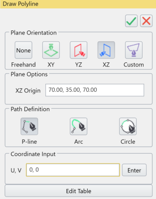
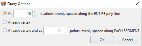
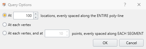
4. A Query options dialog will open, keep the defaults, OK.
   

7.0 Meshing

We will add two mesh refinement regions, one at the bottom surface of foundation and another using mesh refinement region box.

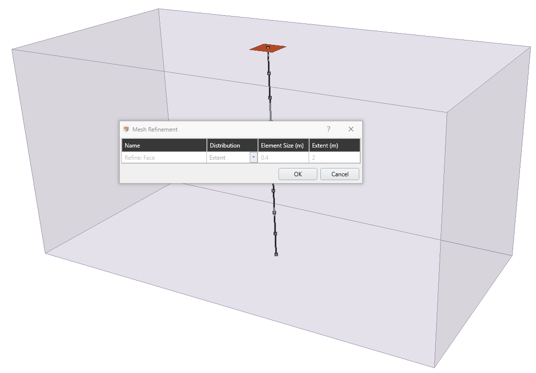
1. To set mesh refinement at the bottom surface of foundation, hide the foundation entity and select the top surface of soil in contact with foundation.
   
2. Select: Mesh > Define Refinement Regions.
   
3. Enter Distribution = "Extent", Element Size (m) = 0.4 and Extent (m) = 2.
   
4. For the mesh refinement region box, deselect all entities and select: Mesh > Define Refinement Regions.
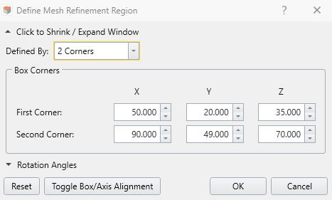
5. A Define Mesh Refinement Region dialog will open. Enter:
   
   1. First Corner (x, y, z) = (50, 20, 35),
      
   2. Second Corner (x, y, z) = (90, 49, 70),
      
6. Click OK.
   
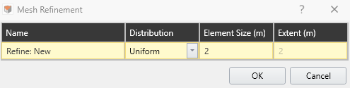
7. Select Distribution = "Uniform". Enter Element Size (m) = 2 and Extent (m) = 2.
   
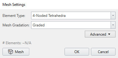
8. Select: Mesh > Mesh Settings
9. Enter Element Type = 4-Noded Tetrahedra and Mesh Gradation = Graded
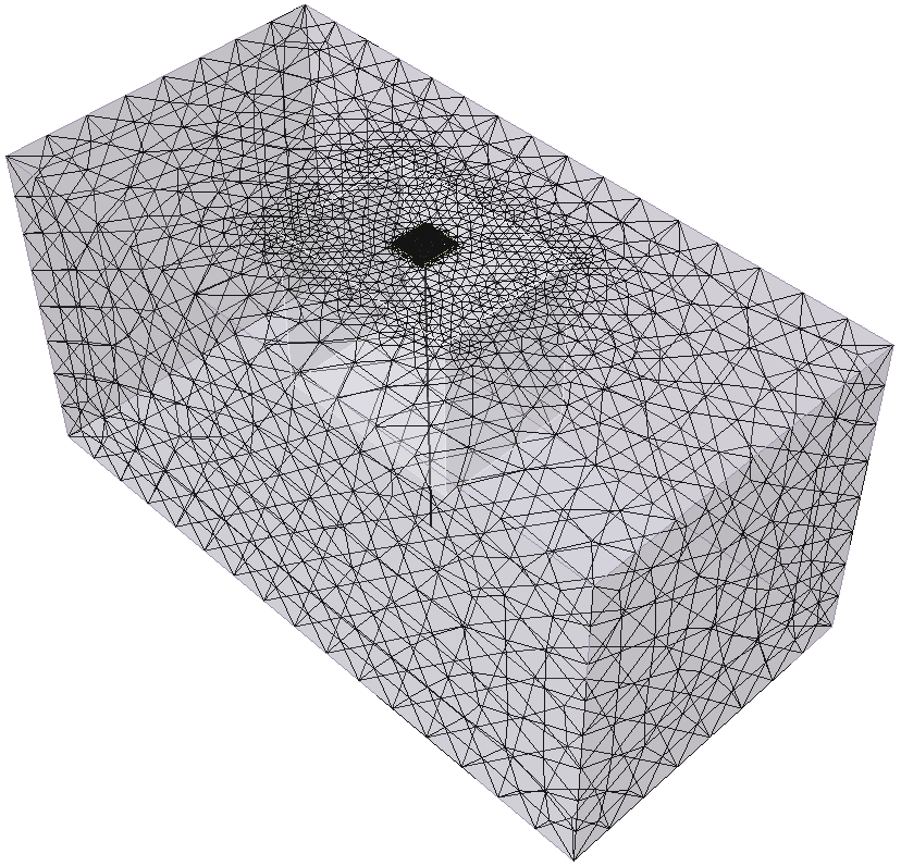
10. Click Mesh to mesh the model.

The mesh is now generated, your model should look like the one below.

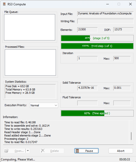
8.0 Computing Results

1. Next, we move to Compute workflow tab . From this tab, we can compute the results of our model.

Before commencing the stress analysis computation, it is recommended to save the final model as a separate file so that you can access the original file anytime.

2. Select File > Save As to save a copy of your model.
   
3. Select Compute > Compute to compute the model.

A warning dialog will appear asking if you would like to compute without restraints. This is because displacement restraints are not applied throughout the entire stages, which is not necessary for this model since Initial element loading for both materials are set to None (meaning that the material is not going to react by field stress nor its own weight) and dynamic boundary condition is already applied to absorb the dynamic load applied. Therefore, it is safe to select Yes to the warning.

9.0 Interpreting Results

9.1 DISPLAYING THE X DISPLACEMENT RESULTS

On the top right corner of the Results tab, you should see two drop-down menus:

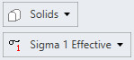
1. Ensure [Solids] is selected from the Element drop-down menu.
2. We will analyze the X Displacement results, so select Data Type > Solid displacement > X Displacement.
   

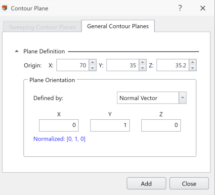
Let’s add a plane contour so we can see some results:

3. Select: Interpret > Show data on plane > XZ Plane
4. Enter Origin (x, y, z) = (70, 35, 35.2), Normal (x, y, z) = (0, 1, 0). Then click Add.
   

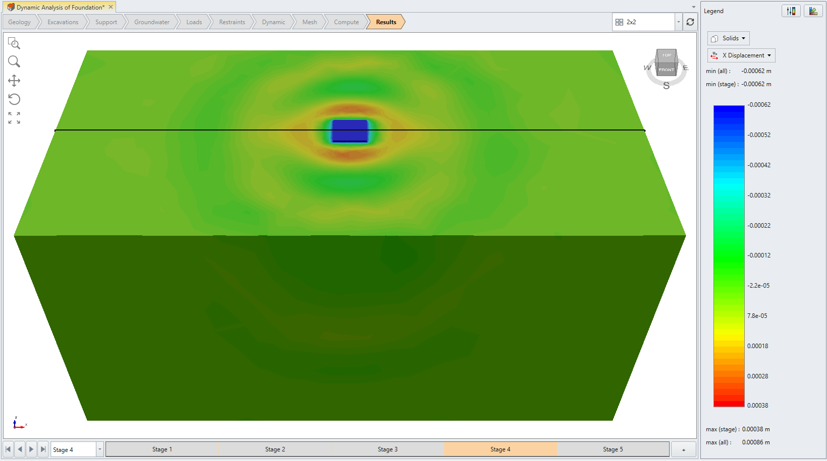
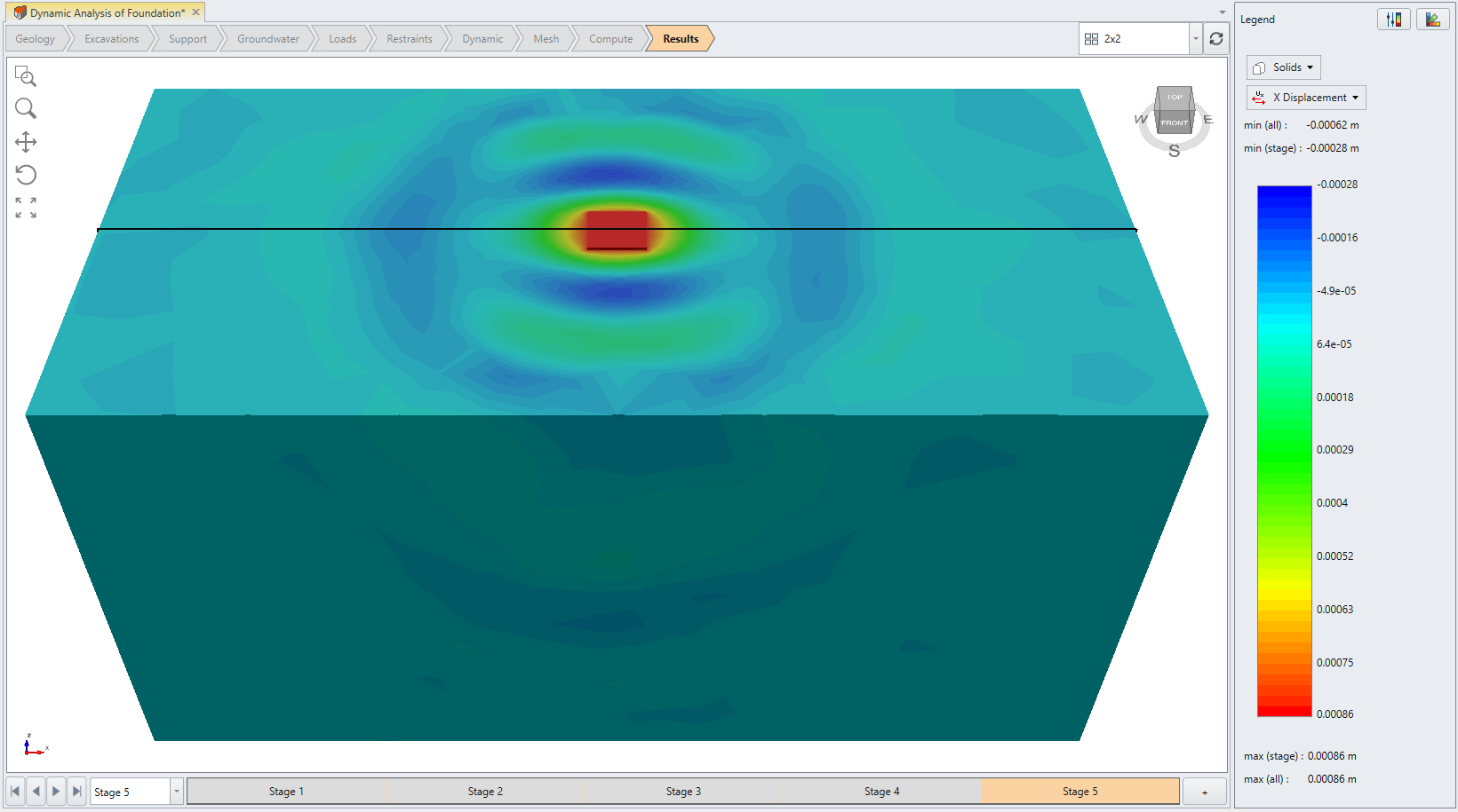
In any given dynamic loading stage (between Stage 2 and Stage 5), the translation of shear wave descending from the foundation down towards the bottom boundary can be observed. The travelling wave is apparent from the alternating blue (cold) and green (warm) zones which represent negative and positive horizontal displacement respectively. Also, toggling through the dynamic loading stages you can observe the formation of a new negative/positive displacement zone foundation oscillates left and right. This motion is the expected soil behavior from a foundation with lateral machine loading acting on it. The x displacement results on XZ contour plane should look like the following (showing shear waves propagating through the ground):

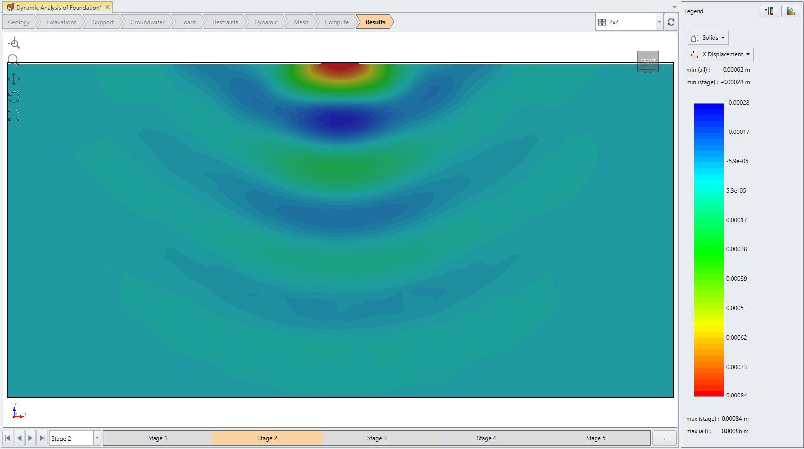
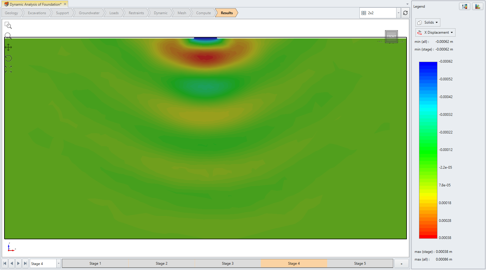
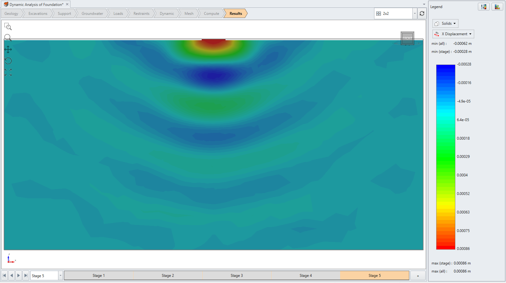
If your model does not look like the figure shown above try toggling off the Exterior Contour layer from the Visibility pane.

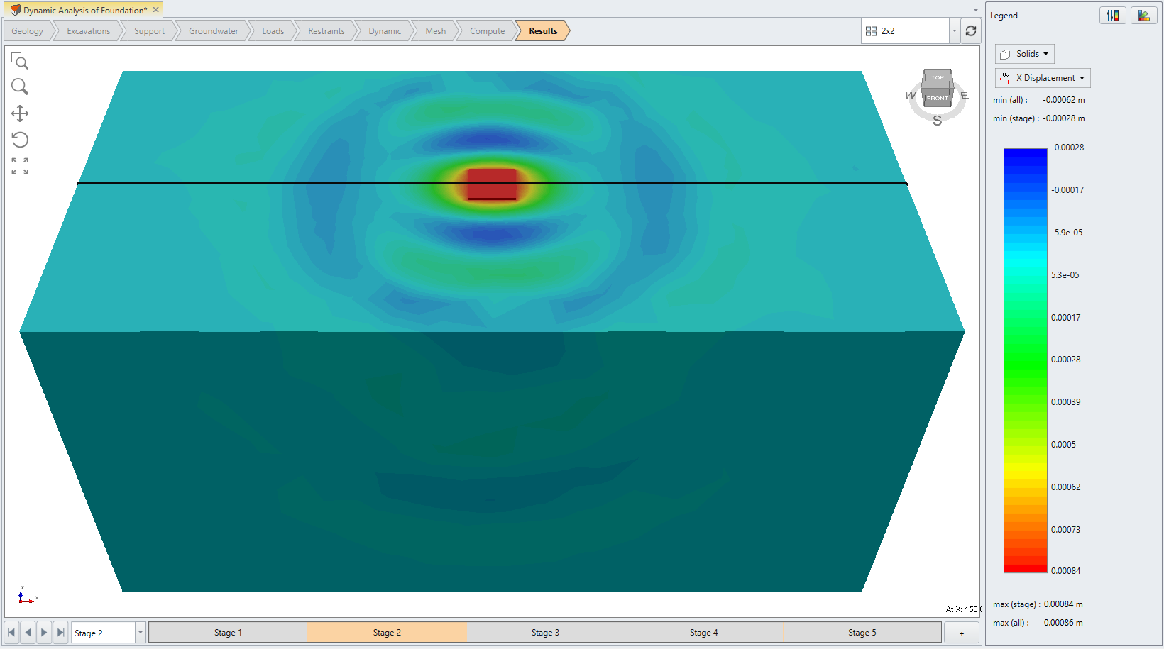
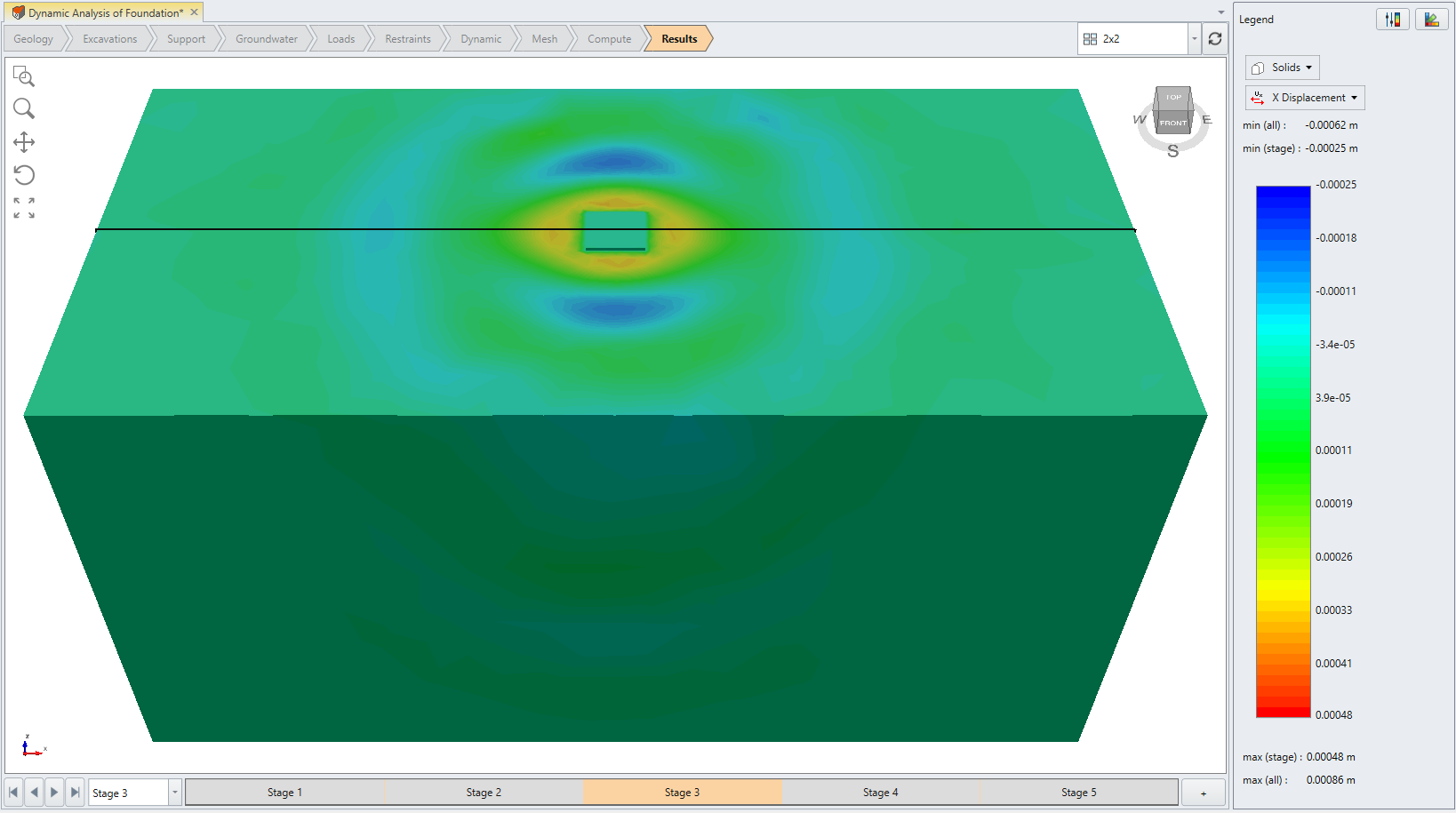
5. Select: Interpret > Show Exterior Contour

On the exterior, you can also see the propagation of the shear waves outwards laterally. The results are shown with auto-range with an exterior contour plot to better illustrate wave propagation from foundation to soil at each stage. The results through the stages should look like the below:

9.2 GRAPHING THE QUERY LINE RESULTS

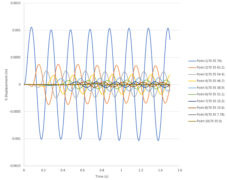
Using a time-query poly line, it is possible to plot the change in kinematic data (displacement, velocity, and acceleration) with respect to time at the location of query points along the line. It can be performed by selecting “Polyline_dynamic” in the visibility pane and selecting [Graph Data] in the properties pane. This opens a new tab with a series of curves (with each curve or data series corresponding to one query point in the time query) on the time-distance plane, plotting the change in X-displacement (normalized by distance) with respect to time. The plotted data corresponds to those collected for the current stage of which the modeling result is displayed. Note that the data ranges for each query point is normalized based on the maximum range of all query data and spacing between query points being plotted to more effectively visualize the relative difference between points at each time interval. If you add only a time query point, the graph is plotted with the original data and is not normalized since it is the only data series that is being plotted.

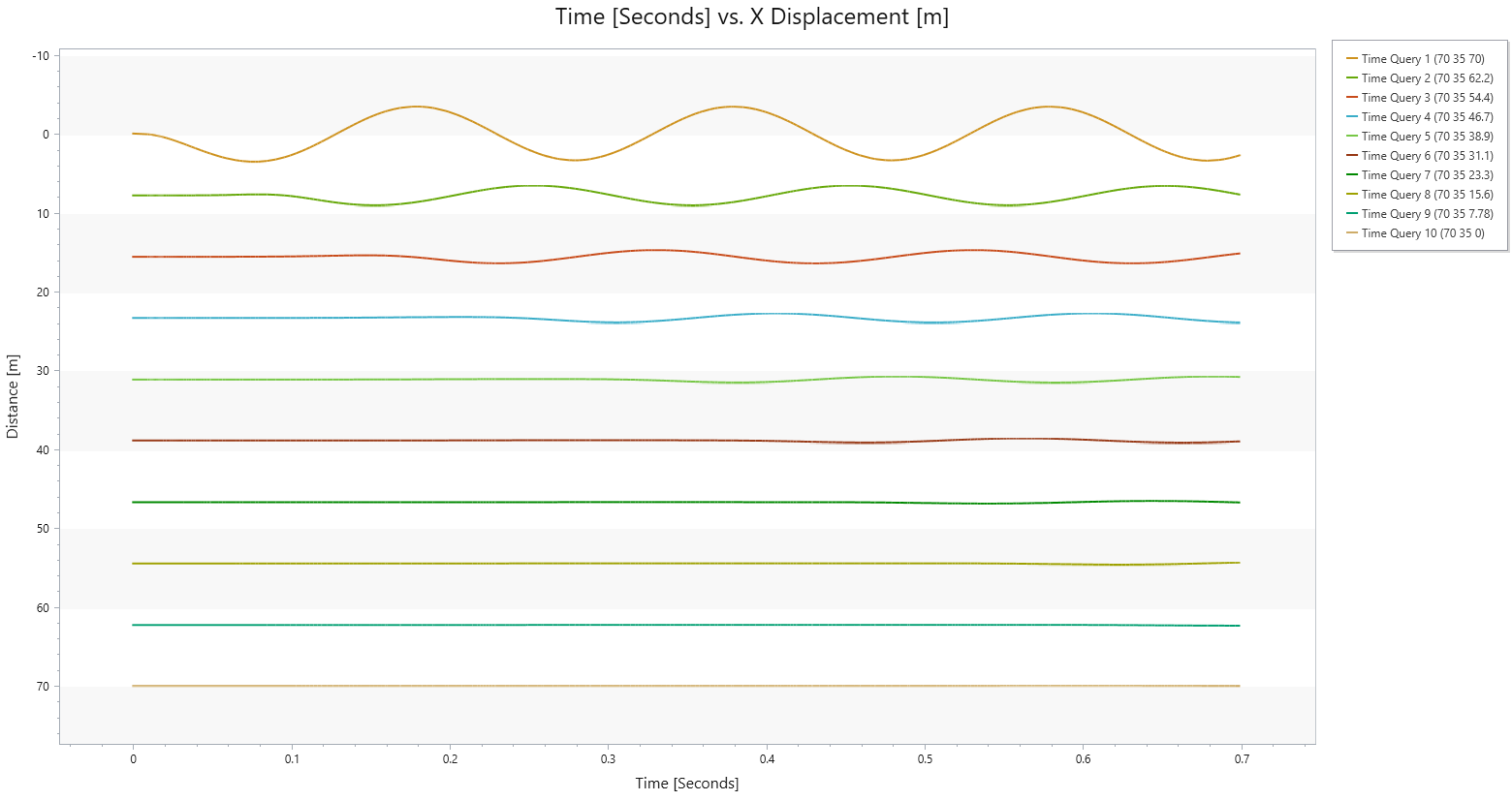
The time query line data for X Displacement for Stage 2 should show the normalized X Displacement at time interval between 0 s and 0.7 s; and Stage 5, 0.75 s and 1.5 s. The results through the dynamic stages should look like the below:

Stage 2:

Stage 5:

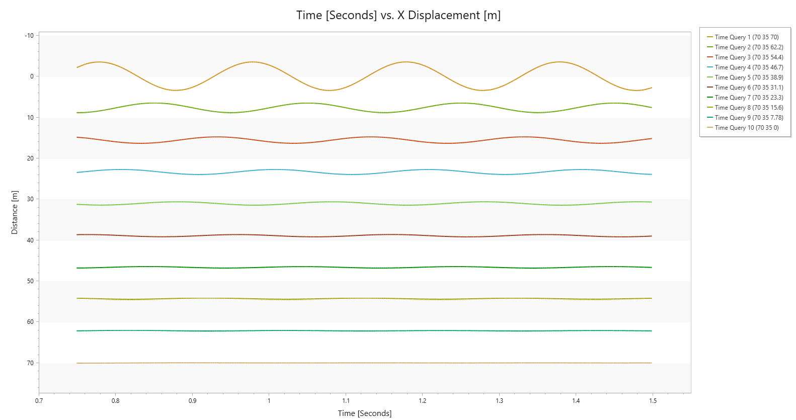
From the generated graphs it is apparent that the amplitude greatly reduces from the motion at the surface to that at the bottom boundary. Comparing the time the peak values occur on the upper query point to the next, it is apparent that the wave takes about 0.12 s to travel 7.8 m. Settings can be adjusted using the pane on the left. Select Change Plot Data to adjust the graph data including the time scale. Other results are available to view as well.

To obtain the query data without normalization being applied, follow the steps discussed above to plot the Time - X Displacement graph at Stage 2.

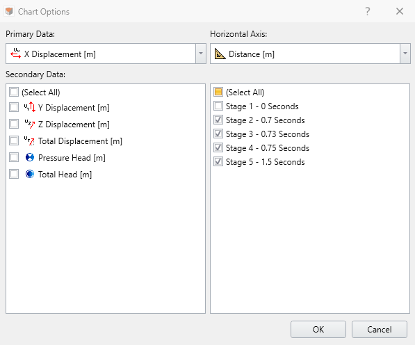
1. Under Chart Options Select [Change Plot Data...]
2. The Chart Options dialog will appear. Check all stages and click OK.
   
   This will show the change in normalized X Displacement throughout the whole stage (From 0 s to 1.5 s).
3. Right-click the anywhere on the graph and select [Copy Data to Clipboard], which copies the data in csv format and can be directly pasted on the Excel spreadsheet to plot scatter graph.

To obtain the plot of the vertical soil profile, the following steps need to be executed:

1. Select: Interpret > Queries > Add Line Query.
2. In the Draw Polyline Pane, draw a polyline along the same polyline used to create time query polyline and select Done.
3. The Query Options dialog will appear appea. Enter 100 locations.
   
4. Select 'Query Line_results' from Visibility Tree and select [Graph Data] from properties pane.
5. Under Chart Options Select [Change Plot Data...]
6. The Chart Options dialog will appear. Keep the Primary Data = X Displacement [m], Horizontal Axis = Distance [m] and under Secondary Data check from Stage 2 to Stage 5. Click OK.
   
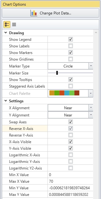
7. Under Chart Options pane on the lefthand side of the graph, under Settings, check Swap Axes and Reverse X-Axis.
   

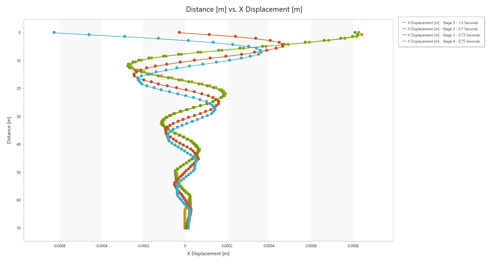
A decaying sinusoidal curve centered about 0 displacement is visible. This wave is the shear wave that causes horizontal movement but travels vertically in the soil model. From the three stages displayed here, the creation of a new peak in the shear wave is evident close to the soil surface. This peak begins to propagate vertically immediately.

This concludes the tutorial.