Anchored Sheet Pile Wall

1.0 Introduction

This tutorial introduces how to model and analyze an anchored sheet pile support system in staged excavation. It uses some of the support features of RS3 such as Liner, joints and bolts for modelling sheet pile and anchors respectively. In the model, the sheet pile walls are installed first. Then, the ground is excavated in different stages. After each stage of excavation, bolts are installed. The model contains two separate layers and the geometry of the model is provided in the initial file.

This example is the extruded version of RS2 - Anchored Sheet Pile Wall. The geometry is imported and extruded in 1 meter in an out-of-plane (z) direction.

All tutorial files installed with RS3 can be accessed by selecting File > Recent > Tutorials folder from the RS3 main menu. The initial file of the tutorial can be found in Anchored Sheet Pile Wall-starting file.rs3v3 and the finished tutorial can be found in the Anchored Sheet Pile Wall.rs3v3 file.

2.0 Starting the Model

After opening the initial file, go to Project Settings:

1. Select: Analysis > Project Settings.

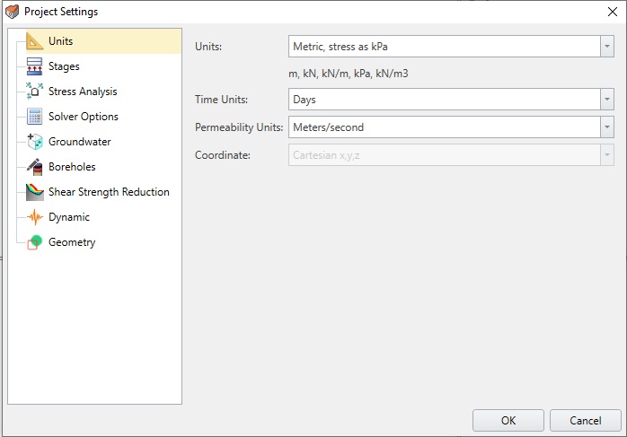
The Project Settings dialog is used to configure the main analysis parameters for your RS3 model.

1. Under the tab [Units], set Units as Metric, stress as kPa. The dialogue should look as shown below:
   
2. Select the [Stages] tab. Enter Number of Stages = 5, with names as shown below. We will be applying different procedures at each stage, so it is important to keep track of the stages by labelling them with relevant names.

Stages	Stage Name
1	Initial
2	Install Sheet Pile Wall
3	Excavate/Install first bolts
4	Excavate/Install second bolts
5	Add Projected Load

After inputting the stages, the dialog should look as follows:

3. Click OK to close the dialog.

3.0 Assigning the Materials

Before we assign the material, we have to create external volumes.

1. Select: Geometry > 3D Boolean > Divide All
   
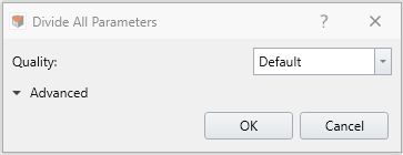
2. Use Default for Quality and click OK.
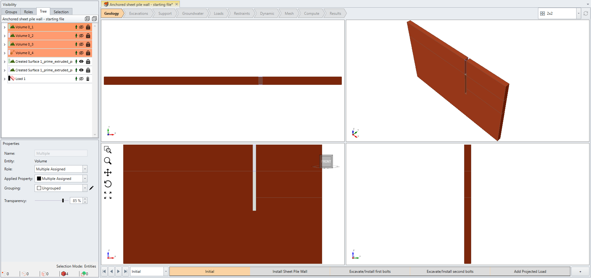
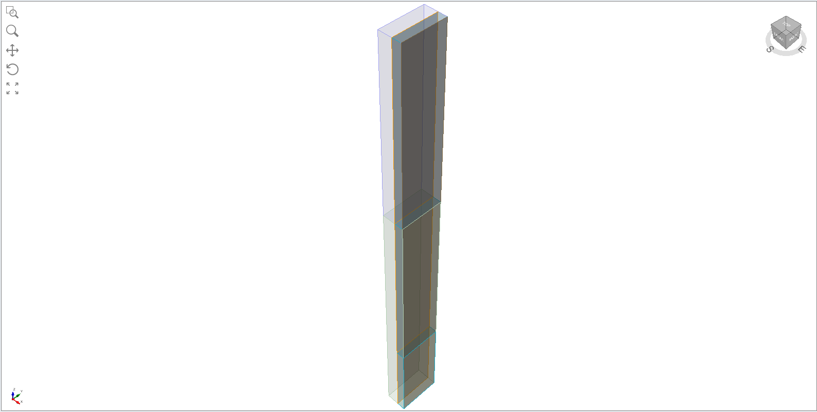
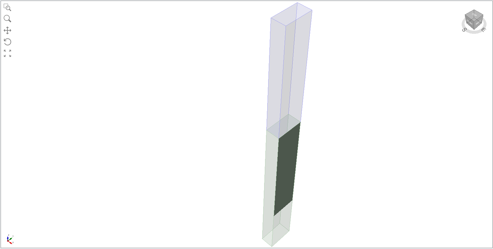
3. You will see the volumes created. Make sure the select entity is selected in toolbar, then select the top three volumes by ctrl + left click on volumes as shown here.
   
   
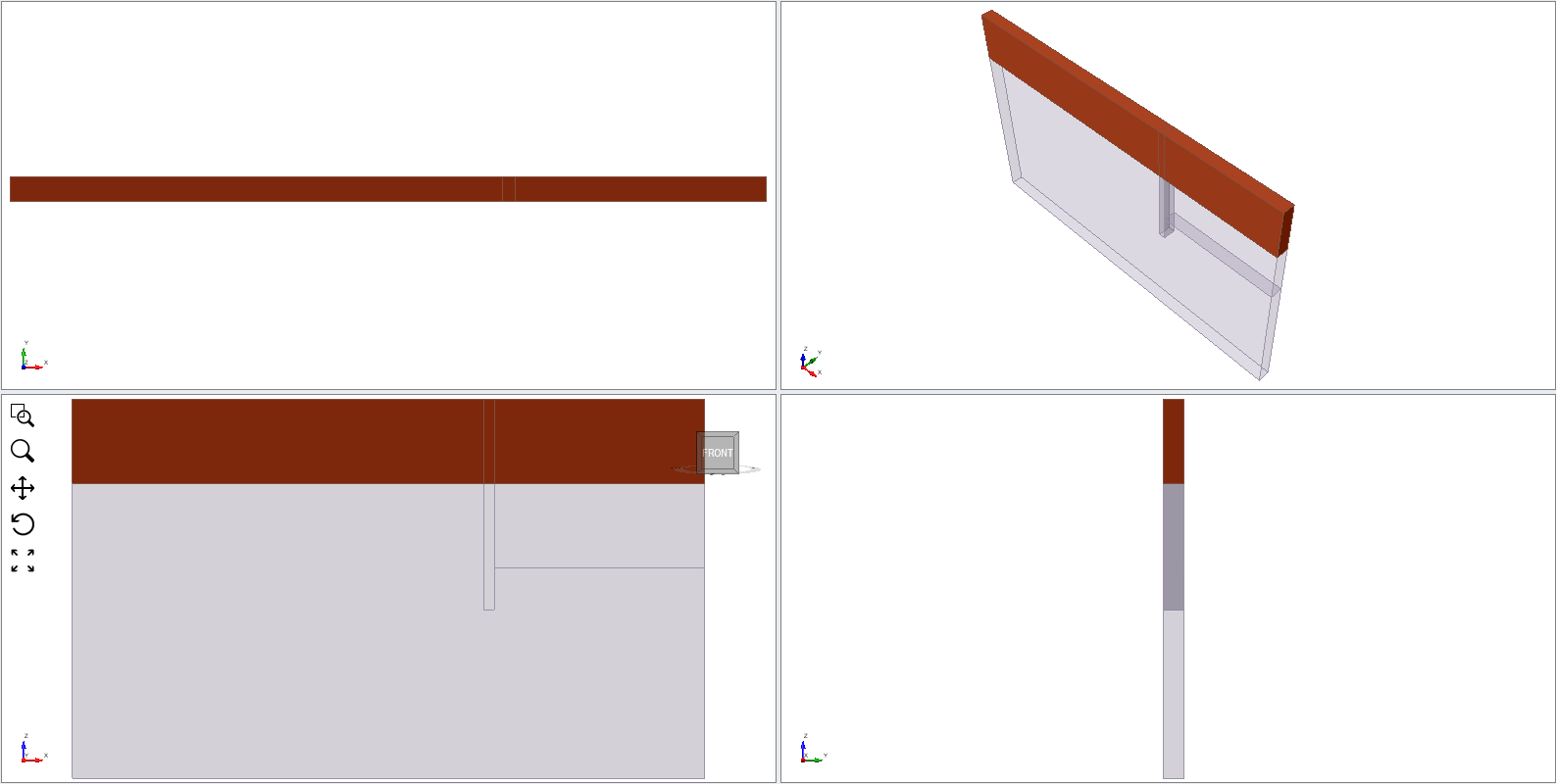
4. The material properties are already provided in the model. Go to properties pane under visibility tree and select Sand. Alternatively, you can also select Materials > Assign Properties.
   
   
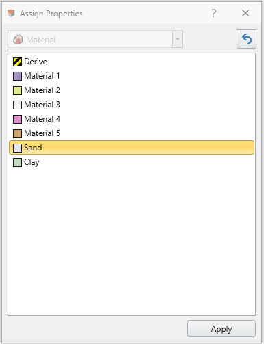
5. Select Apply then you will see the materials are applied on the top volumes.
6. Similarly, we will follow the same procedure for the next bottom layers. Ctrl + left click on bottom volumes and apply Clay property.
   
   
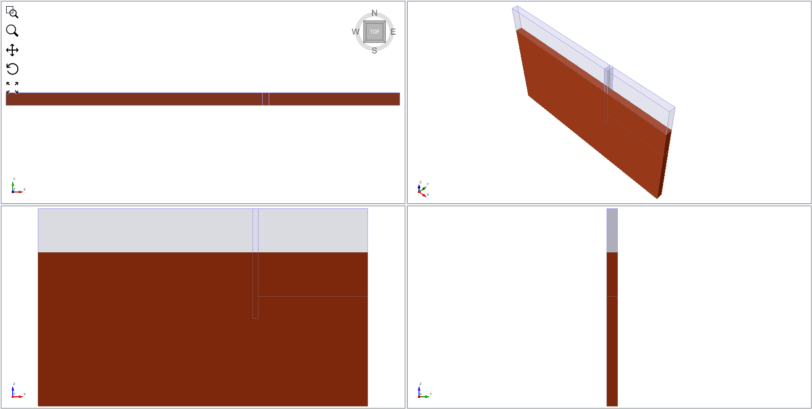
7. Select Apply. Then you will see that materials are applied to two layers as shown below:
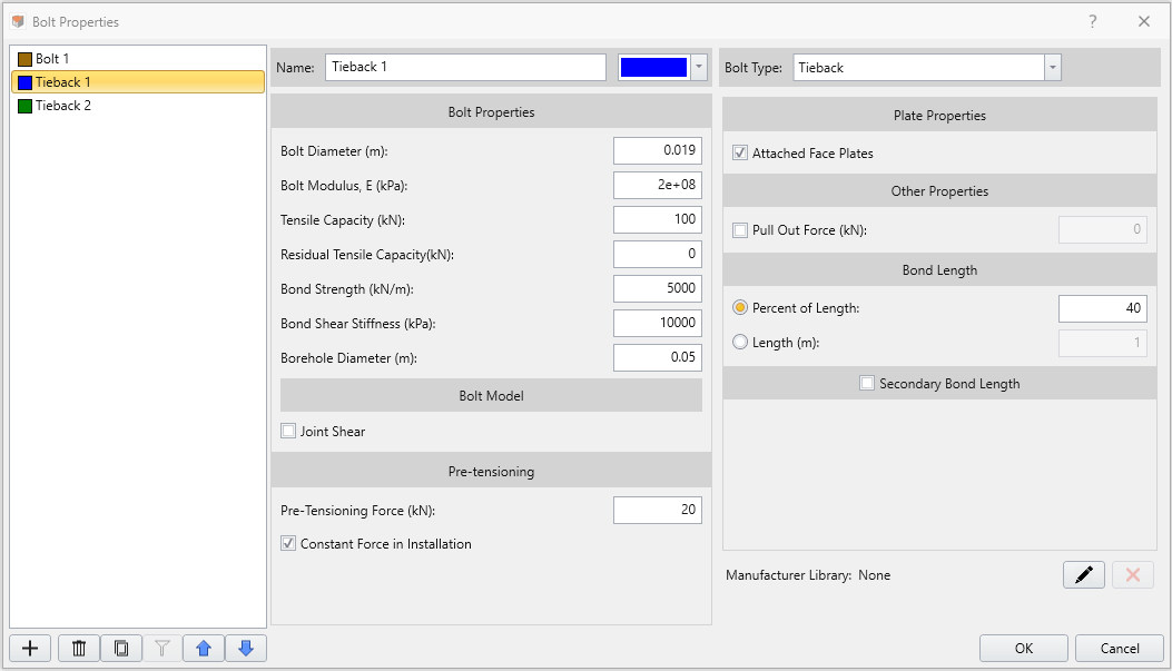
8. We will now assign staged excavation. Select the Volume 0_4 under the Visibility Tree.
   
9. Select the third stage 'Excavate / Install first bolts' and change the Applied property to No Material in the properties pane.
   
10. Next, Select the volume below (Volume 0_3)
11. Select the fourth stage 'Excavate / Install second bolts' and change the Applied property to No Material in the properties pane.

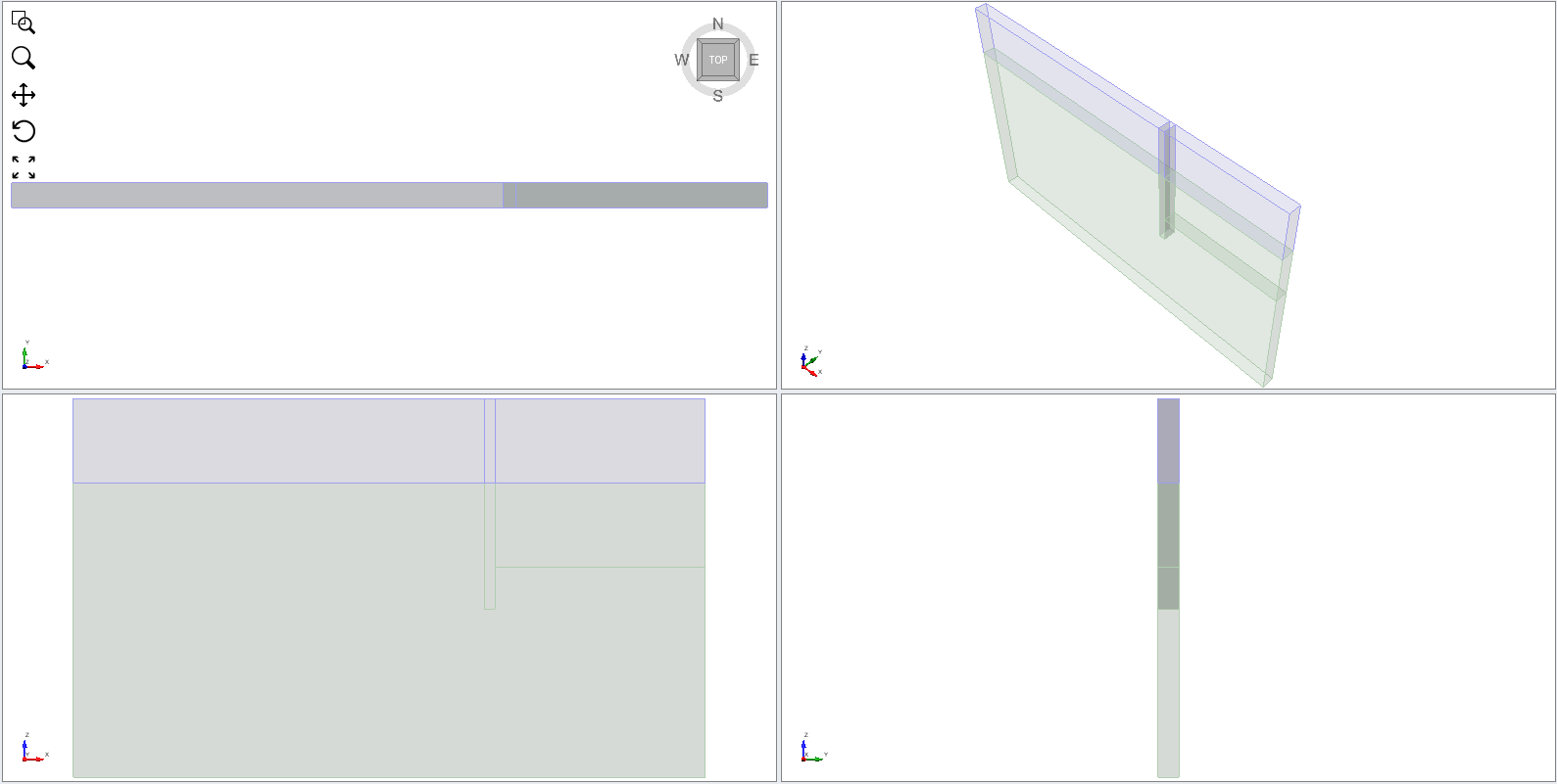
When you click on different stages, you will notice the excavation volume in stages 3 and 4. Now we will move onto supports.

4.0 Defining the Lining Composition

Select: Support > Liners > Defining the Lining Composition

The Lining Composition dialog opens, providing a space to define and save different lining compositions including the Install/Remove stage controls. The tutorial project file has the composition pre-defined as shown below.

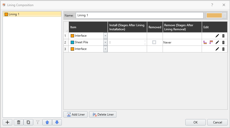
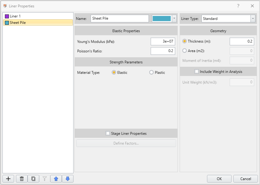
1. The edit icons under Edit column for each layer navigates to its property dialog. The interface property and the liner property must be defined as below

5.0 Assigning the Lining Composition / Bolts

Before we assign the support, we will hide some volumes of the geometry to make it easier for us to assign the liner.

1. Select the following volumes and hide the volumes by selecting the icon next to entity list under Visibility Tree.

5.1 Install Sheet Pile

Navigate to Support workflow tab

1. You will then see the small column of volume is left in the modeler. Set the selection mode to 'Face selection' and ctrl + left click on the three surfaces facing the excavation volume as shown (You can maximize the Perspective view port by double clicking like below).
   
   
2. Then, select Support > Liners > Add Lining.
3. Under Staging, set Install at stage to the 'Install Sheet Pile Wall' stage.
   
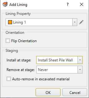
4. Click OK
5. Navigate to Install Sheet Pile Wall stage you will see the liner is applied on the surface as shown below:
   

5.2 Defining/Assigning Bolts

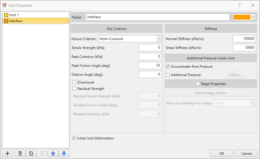
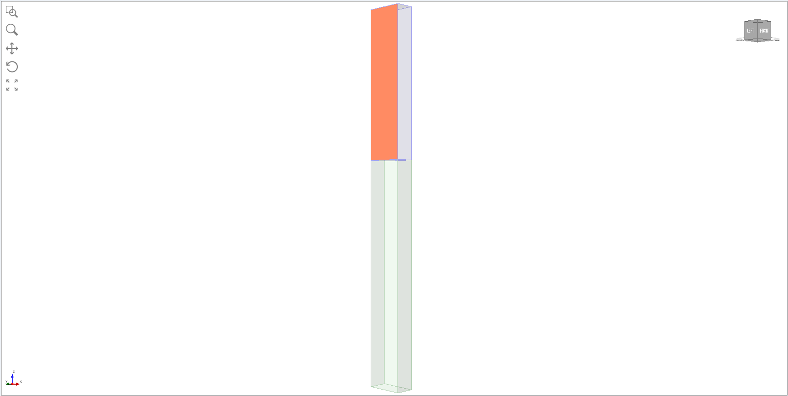
Before applying the bolts to our model, we will first check the bolts properties.

1. Select: Support > Bolts > Define Bolts.
2. Select the Tieback 1 and you will see the following material property shown. Make sure the Attached Face Plates option under Plate Properties is checked:
   
   
3. Click OK. Now we will use this bolt to assign it to our liner layer.
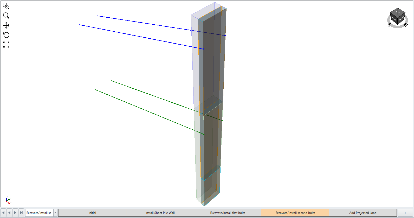
4. Hide the lining entity and select the top right surface (same surface selected for sheet pile installation) as shown below.
   
   
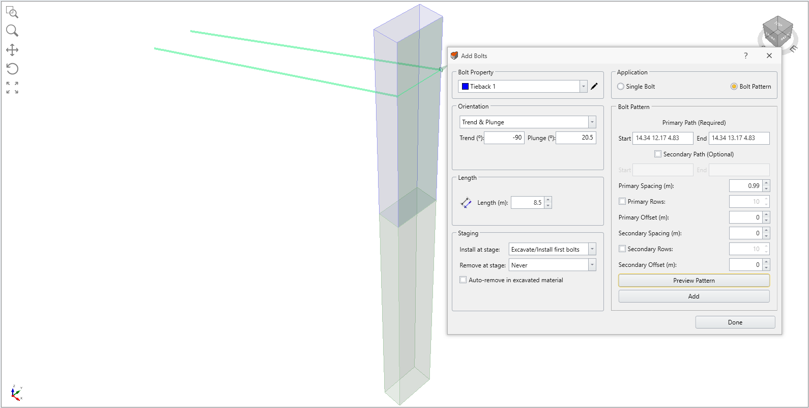
5. Select Support > Bolts > Add Bolts to Surface. Make sure the Tieback 1 is selected under bolt properties. We will assign bolt with the following material property:
   • Trend & Plunge : -90 deg Trend / Plunge 20.5 deg.
   • Length: 8.5 m
   • Install at stage: Excavate / Install first bolts
   • Remove at stage: Never

Primary path inputs are:

• Application: Bolt Pattern
• Primary path (required): Start: (14.34 12.17 4.83) and End (14.34 13.37 4.83)
• Primary spacing (m): 0.99 m * (we set it at 0.99 meters because the extruded model is 1m and the bolt will only show one side of support if 1 meter is entered)
• Primary offset (m): 0 m
• Secondary Spacing (m): 0 m
• Secondary offset (m) : 0m
6. Select Preview Pattern
   
   
7. Click Add > Done

To assign the second set of bolts, select the surface below

1. Select: Support > Bolts > Add Bolts to Surface. Select Bolt 2 under bolt property. We will assign bolt with the following material property:
   • Trend & Plunge : -90 deg Trend / Plunge 20.5 deg.
   • Length: 8.5 m
   • Install at stage: Excavate / Install first bolts
   • Remove at stage: Never

Primary path inputs are:

• Application: Bolt Pattern
• Primary path (required): Start: (14.34 12.17 0.83) and End (14.34 13.37 0.83)
• Primary spacing (m) : 0.99 m
• Primary offset (m): 0 m
• Secondary Spacing (m): 0 m
• Secondary offset (m) : 0m
  
2. Select Add > Done.
3. Navigate to Excavate/Install second bolts stages, all support elements will be shown:
   

6.0 Add Projected Loads

We will now add the load on top of the surface as shown below.

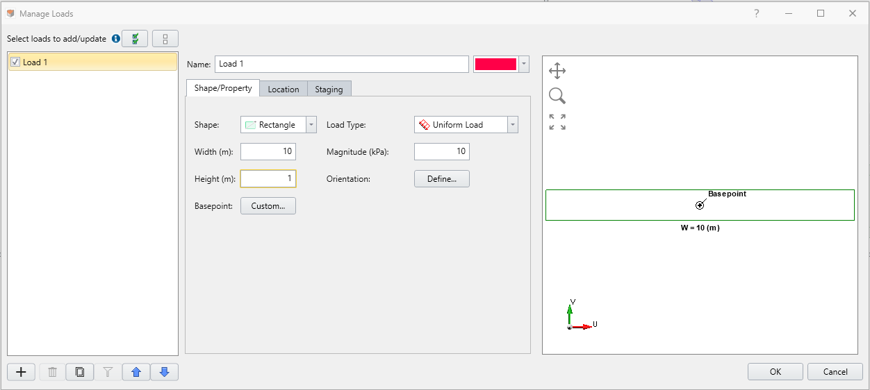
1. Select: Loads > Define Projected Loads.
2. Under Manage Loads dialog, enter following values:
   
   • Width = 10 m
     
   • Height = 1 m
   • Magnitude = 10 kPa
     
3. Select Staging tab, and set Install at stage: Add Load and leave Remove at stage: Never. Click OK.
   

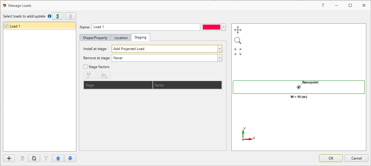
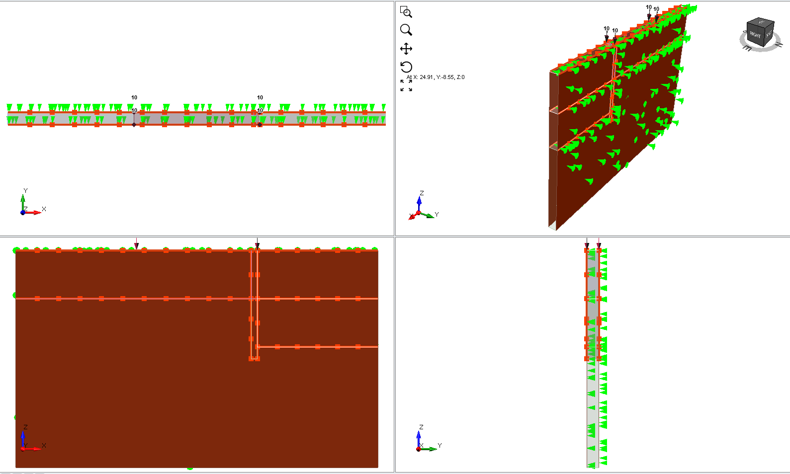
Navigate to Add Projected Load stage, you will see the load applied as shown below:

7.0 Restraints

We will now add restraints to the model.

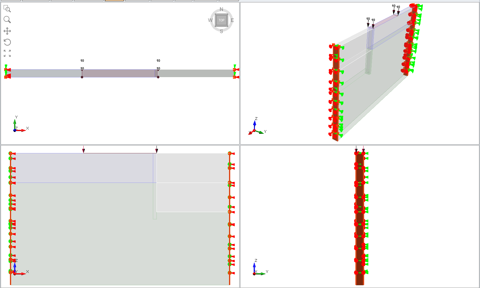
1. First, make sure only the sides of the thin surfaces are selected in the XZ plane.
2. Select: Restraints > Add Restraint / Displacement > Restrain Y.
   
3. Then, select the other surfaces in the YZ direction and then add restraint in XY directions.
4. Select: Restraints > Add Restraint / Displacement > Restrain XY.
   
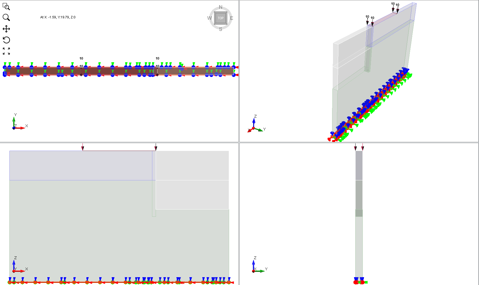
5. Lastly, select the bottom layer (XY plane) and select Restrain XYZ.
6. Select: Restraints > Add Restraint / Displacement > Restrain XYZ.
   

8.0 Meshing

1. Next, we move to the Mesh workflow tab.

Here we may specify the mesh type and discretization density for our model.

1. Select: Mesh > Mesh Settings
2. For this tutorial, we will use a default setting,4-noded tetrahedra graded mesh.
   
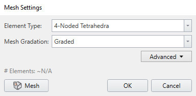
3. Click Mesh to generate the mesh, and then OK.
   

The mesh is now generated, your model should look like the one below.

Now we move on to computing the results.

9.0 Computing Results

9.1 COMPUTING THE MODEL

1. Next, we move to Compute workflow tab
2. From this tab, we can compute the results of our model. First, save your model: File > Save As.
3. Next, you need to save the compute file: File > Save Compute File. You are now ready to compute the results.
4. Select: Compute > Compute
   

10.0 Interpreting Results

10.1 DISPLAYING THE RESULTS

1. Next, we move to Results workflow tab
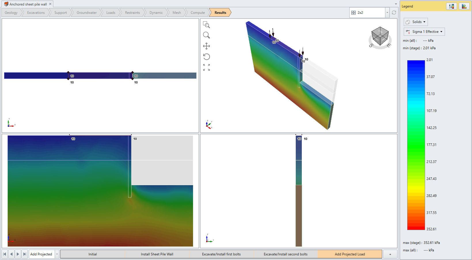
2. Navigate to Add Projected Load stage
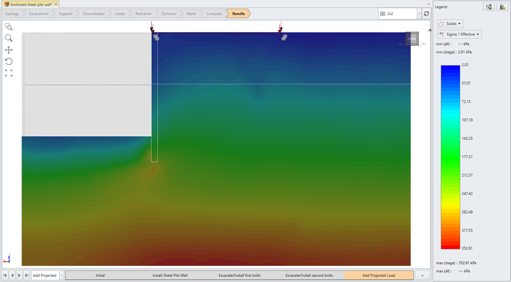
3. Select Interpret > Show Exterior Contour, the Sigma1 Effective stress contour will be rendered:

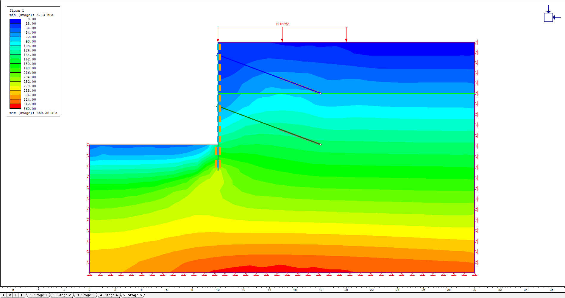
Below shows a comparison between the Sigma 1 contour diagram obtained from RS3 and the equivalent model from RS2 (See: RS2 Tutorials | Anchored Sheet Pile Wall), showing close agreement.

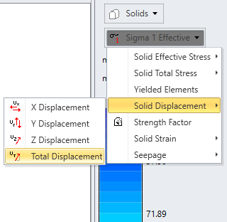
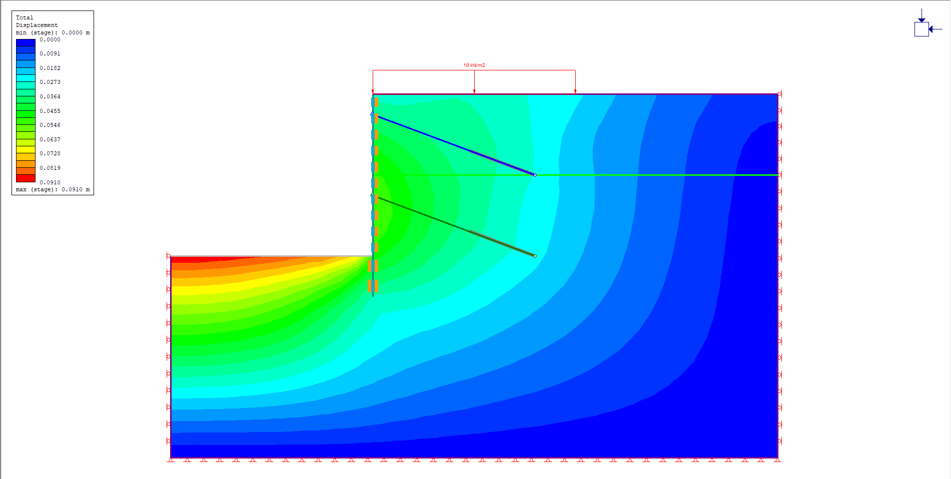
1. Next, switch the data type to Total displacement.

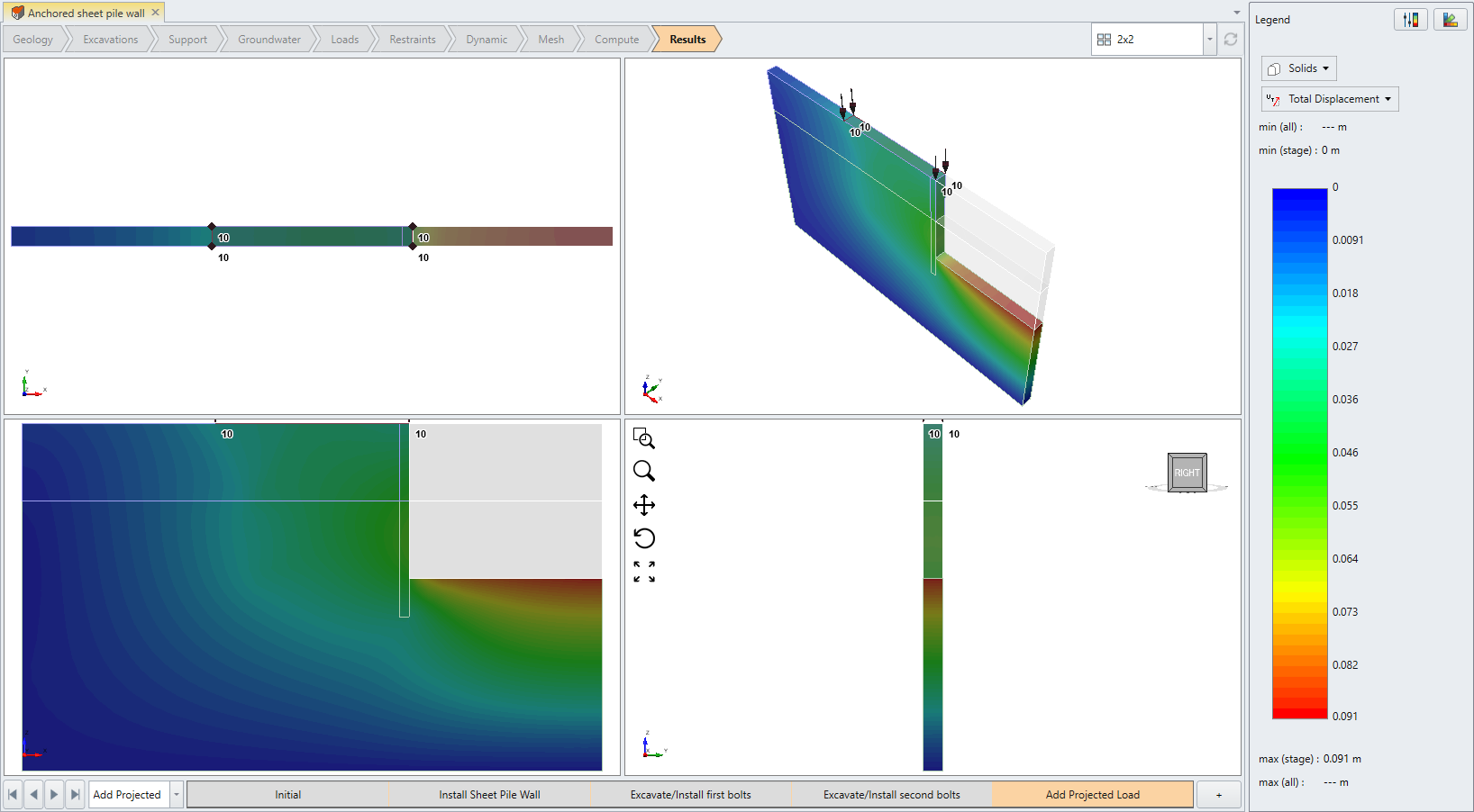
Below is the Total Displacement contour from RS2, showing close agreement to that from RS3.

This concludes the Anchored Sheet Pile wall tutorial.