Groundwater Seepage Analysis
1.0 Introduction
This tutorial introduces groundwater seepage analysis in RS3. The model used in this tutorial consists of a basic, steady-state groundwater seepage analysis. In the tutorial, we will cover adding groundwater boundary conditions as well as ponded water loading. This tutorial will focus on the results of the analysis; after a groundwater seepage analysis is computed, the results (pore pressures) are compared in Slide3, RS2 and RS3.
2.0 Import Slide3 to RS3 for Pore Water Pressure Analysis
We will be performing a groundwater seepage analysis using RS3. RS3 uses Finite Element Methods to run seepage analysis using groundwater boundary conditions which is different from Slide3. Here we will demonstrate how this can be done with the geometry created from Slide3.
First, we will import the Slide3 model to RS3.
- Select File > Import > Import Slide3 Project

- Select Steady state seepage_Slide3.slide3m2 within the Groundwater Seepage analysis-RS3 final tutorial folder. Click Open.
- De-select Generate Mesh and set Auto Restraints to None.
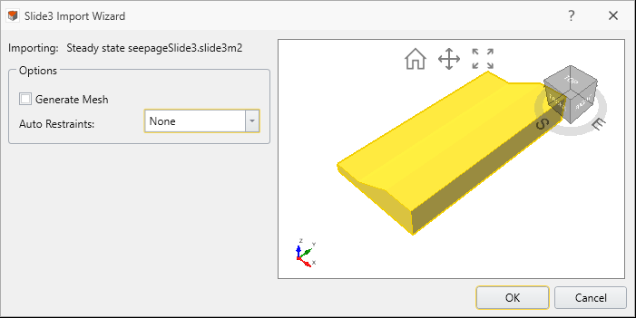
- Click OK.
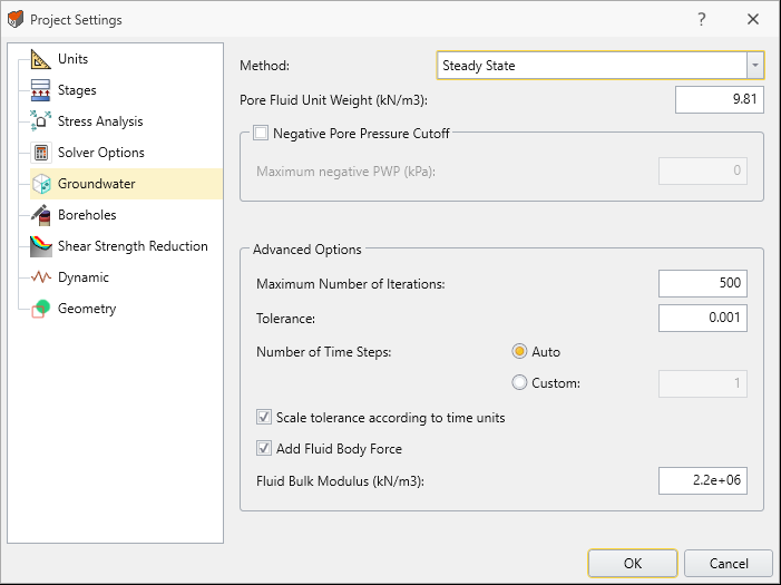
- Go to Project Settings by selecting Analysis > Project Settings

- Under the Groundwater tab, change the method to Steady State as shown below:
- Under the Shear Strength Reduction tab, when a model is imported from Slide3 the Determine Strength Reduction Factor checkbox is turned on automatically. Since an SSR analysis is not part of the scope for this tutorial, turn the Determine Strength Reduction Factor checkbox off.

3.0 Applying Groundwater Boundary Conditions
We will now assign groundwater boundary conditions to the model.
- Select the Groundwater workflow tab

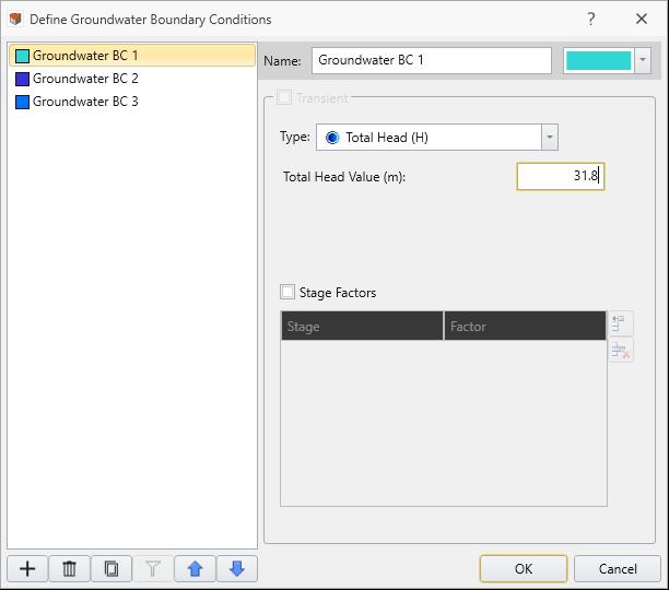
- Select Groundwater > Define Groundwater Boundary Conditions

- Add two more layers of groundwater boundary condition by selecting the Add button
 in the bottom-left side of the dialog.
 - For Groundwater BC 1, select Type = Total Head (H) and enter Total Head Value (m) = 31.8 as shown below:
- For Groundwater BC 2, select Type = Total Head (H) and enter Total Head Value (m) = 26 as shown below:

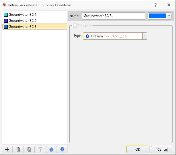
- For Groundwater BC 3, select Type = Unknown (P=0 or Q=0)
- Click OK to save and close the dialog. Now we will assign these boundary conditions to the geometry.
- Select Edit > Selection Mode > Faces Selection
 or select these options from the toolbar.
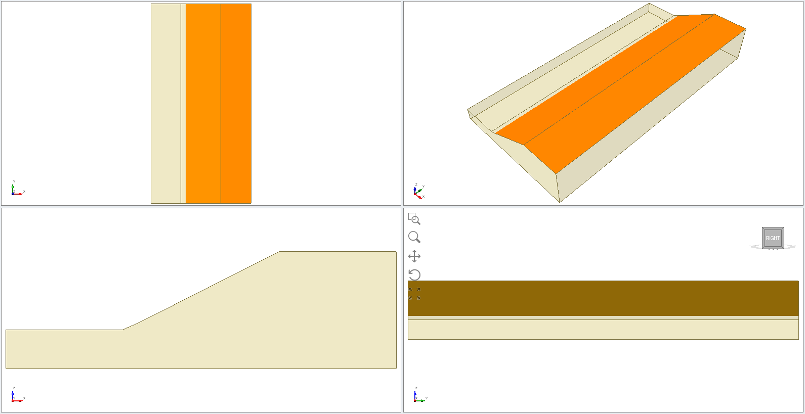
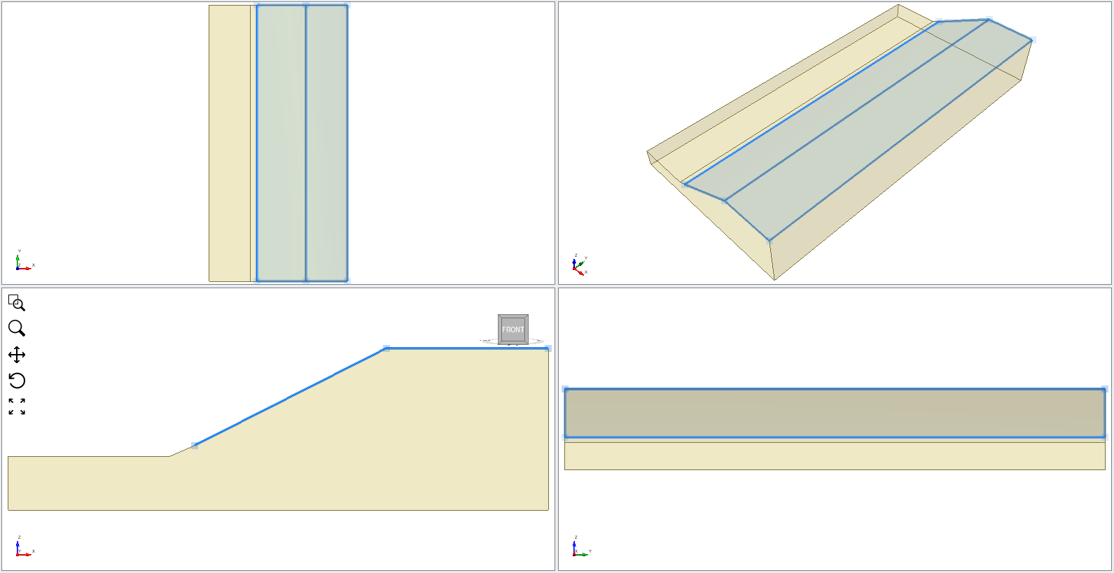
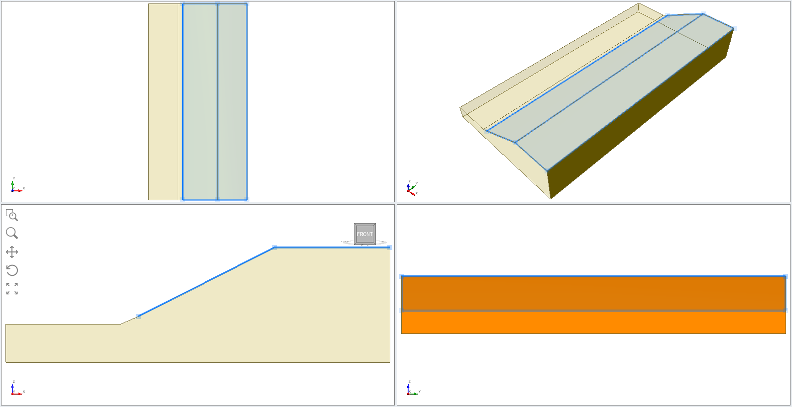
 - Select the top surface and the top portion of the slope of the geometry.
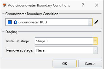
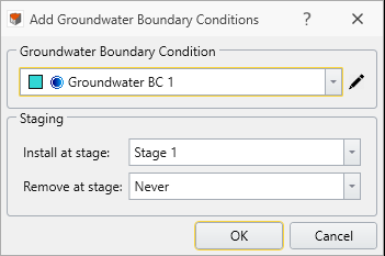
- Then select Groundwater > Add Groundwater Boundary Conditions. Use the drop-down to assign Groundwater BC 3 to those surfaces.
- Click OK. You should see the following groundwater boundary conditions as shown below:
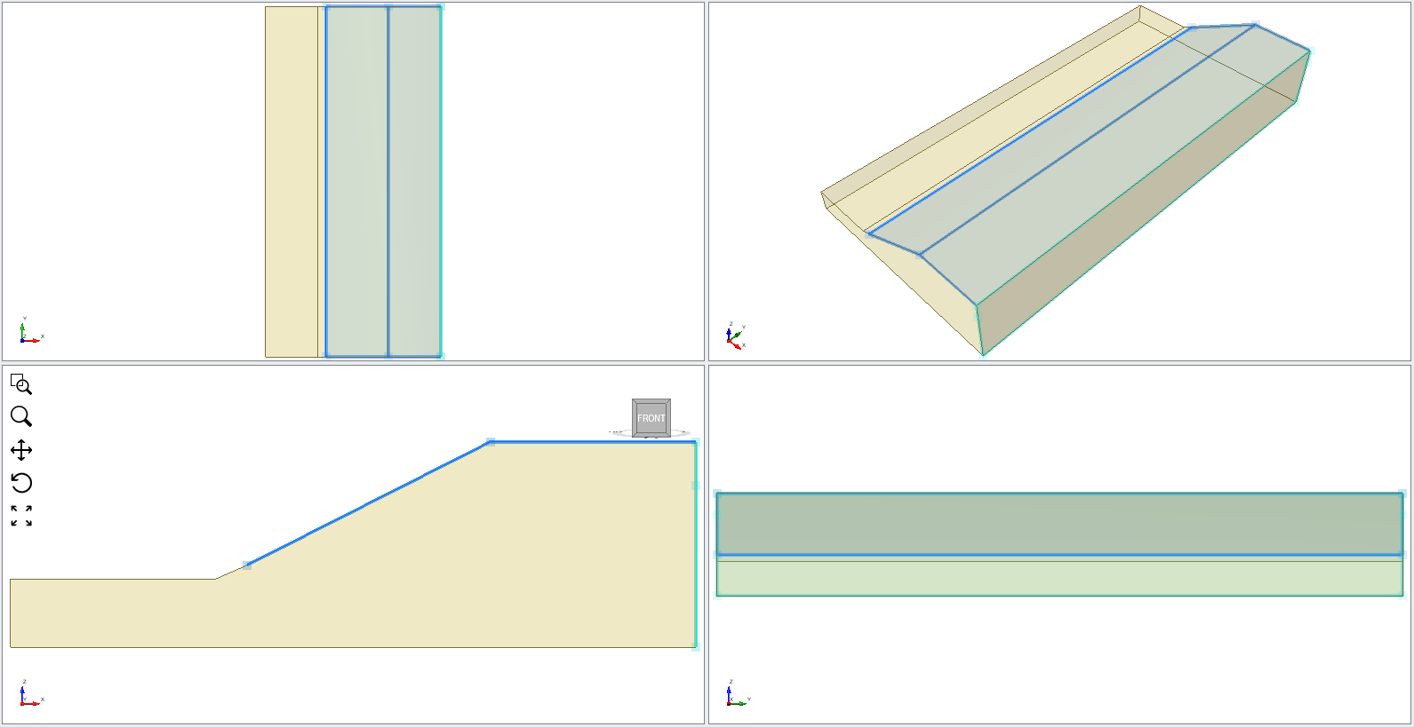
- Now, select the back end of the surface (or the surface on a higher slope).
- Then select Groundwater > Add Groundwater Boundary Condition. Under the drop-down menu for the Boundary Condition, select Groundwater BC 1.
- Click OK, the model should look like the following:
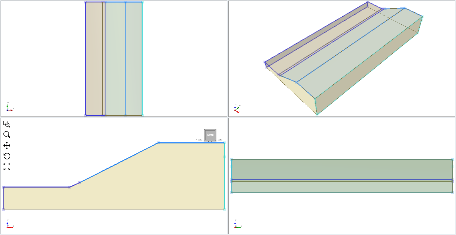
- Select three surfaces at the front (lower end) and front surface as shown in the figure below:

- Then select Groundwater > Add Groundwater Boundary Condition. Under the drop-down menu for the boundary condition, select Groundwater BC 2.

- Click OK.
The model should look like the following:
4.0 Applying Load
- Select the Loads workflow tab
 . Ponded water needs to be applied as a load to account for the weight of water.
 - Select two surfaces at the front (lower end) as shown in the figure below:

- Then select Loading > Add Loads to Selected.
- Under the drop-down menu for the load type, select Ponded Water Load. Enter Total Head = Constant and 26 (m).
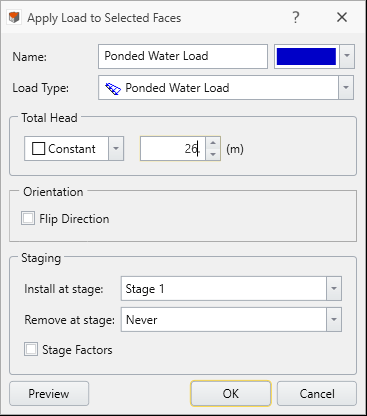
- Click OK.
5.0 Applying Boundary Conditions
- Select the Restraints workflow tab

- Select Restraints > Auto Restrain (Surface)

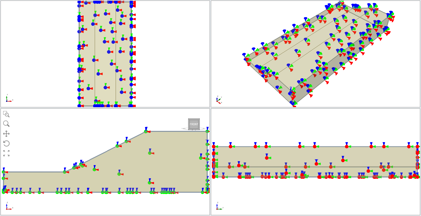
The model should look like this.
6.0 Mesh
- Select the Mesh workflow tab

- Select Mesh > Mesh Settings

- Keep the mesh setting to the pre-defined values.
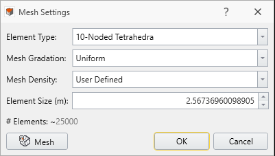
- Select Mesh
 . Then click OK. You should see the following:
7.0 Compute for Seepage Analysis
- Select the Compute workflow tab
 . You are now ready to compute the results.
 - Select Compute > Compute

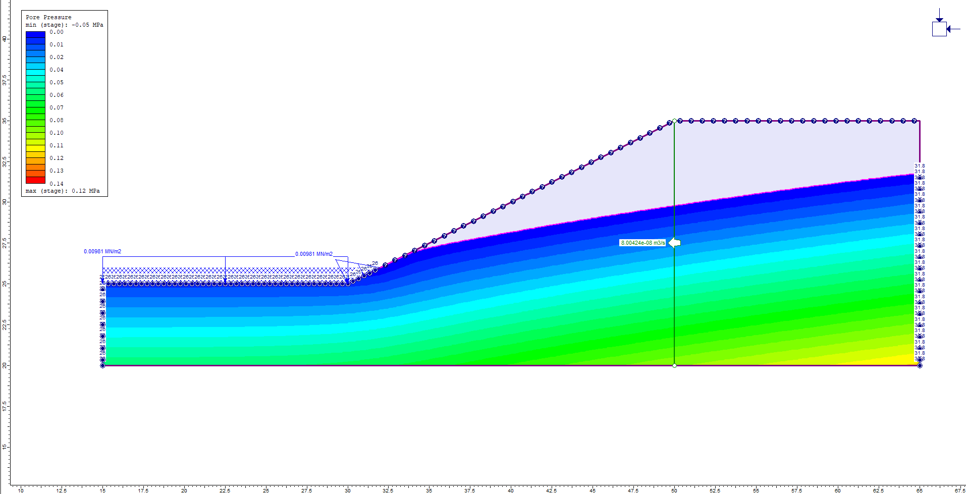
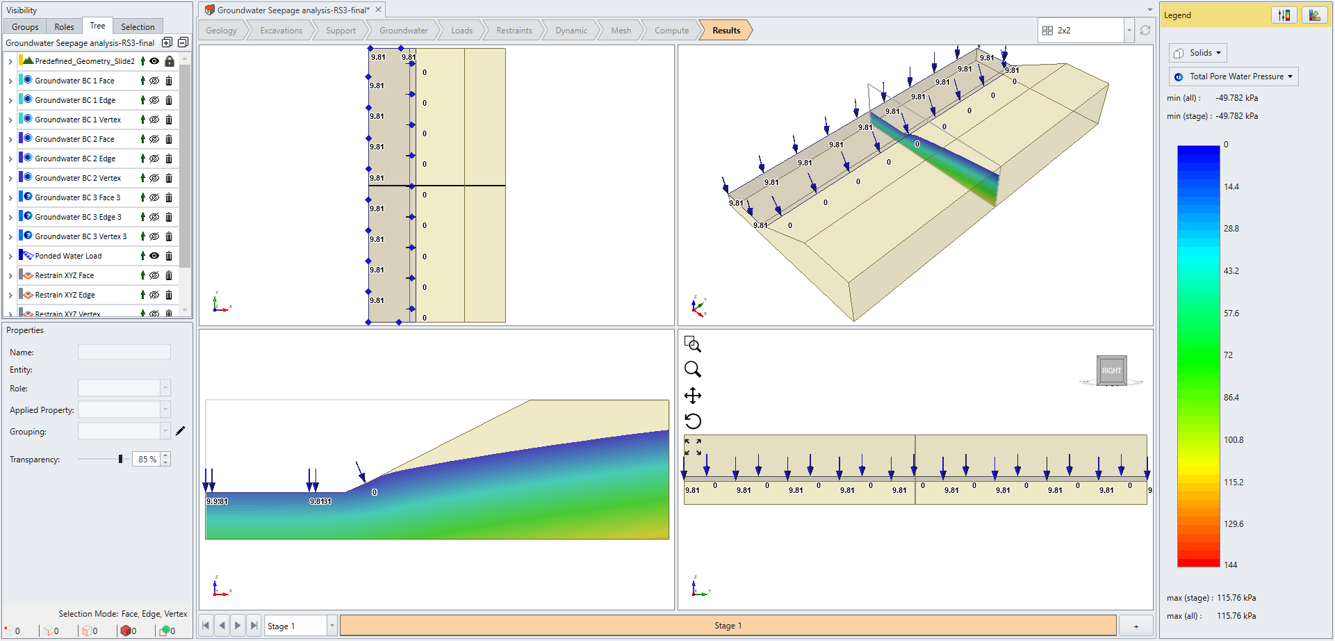
8.0 Results
- Select the Results workflow tab

- Select Interpret > Show Data on Plane >XZ.
- Use the default settings.
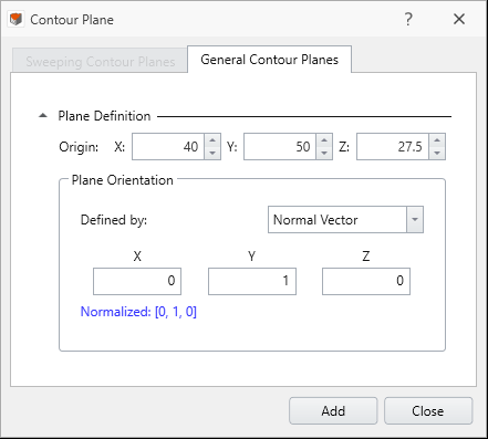
- Select Add.
- Go to the Legend, and under Solids, select Total Pore Water Pressure.
- For comparison with Slide3, RS2 and RS3 results, we will choose Pore Water Pressure.
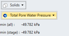
- For comparison with Slide3, RS2 and RS3 results, we will choose Pore Water Pressure.
- Click Contour Options

- Under the contour range section, select 0 to 144 for the Custom Range as also shown below. Also, select Interval Count = 24.

- Click OK to save and close the dialog.
Using the analysis results from RS3, we will now export the water pressure grid from RS3 to Slide3.
- Select File > Export > Export Pore Water Pressure to Slide3.
- Save the file with the title of the project (pore water pressure grid slide3.pwp3). We will import this file to Slide3.
We can compare the result from RS2 with the same setting. We can see that the two models show a close agreement. The RS2 model can be found from RS2 Tutorial - Finite Element Groundwater Seepage.