Application of Discrete Fracture Networks

1.0 Introduction

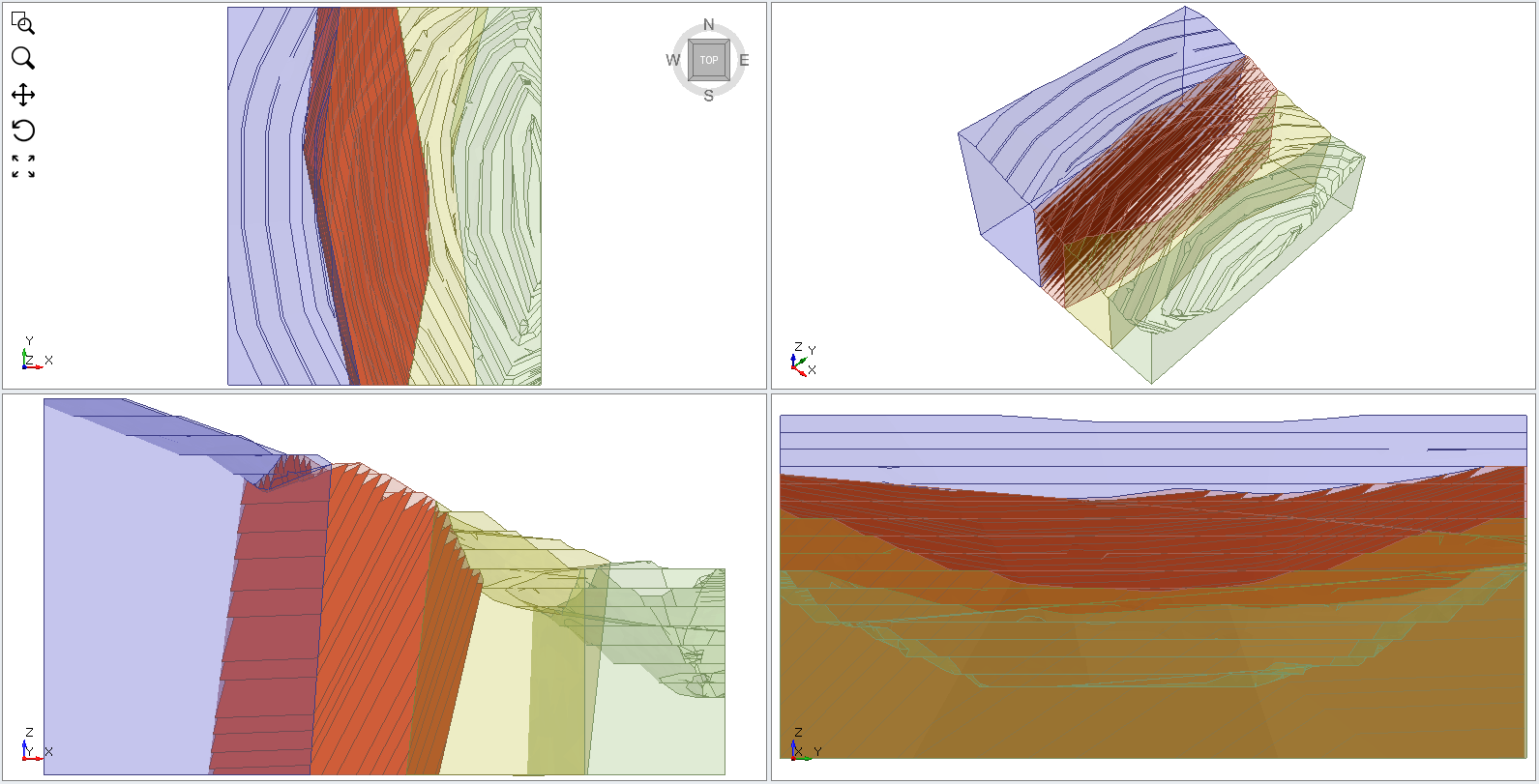
This tutorial demonstrates how to apply Discrete Fracture Network (DFN) to the RS3 model. The DFN approach for modeling fractured rock masses refers to explicit representation of fractures forming a network. This tutorial covers the use of DFN to represent a joint set applied to a sector of an open pit mine, which consists of sandstone, schist, shale, and siltstone. The joint set dips at 63 degrees, dipping towards 259 degrees (in near opposite direction from the slope).

All tutorial files installed with RS3 can be accessed by selecting File > Recent > Tutorials folder from the RS3 main menu. The initial file of the tutorial can be found in DFN application - starting file.rs3v3 file and the finished tutorial can be found in the DFN application - final.rs3v3 file.

2.0 Starting the Model

1. Select File > Recent > Tutorials from the menu.
2. Open the starting file DFN application - starting file.rs3v3.

The model should have initial project settings and material properties of external volume already defined for the user.

1. Select: Analysis > Project Settings
2. The Project Setting dialog is used to configure main analysis parameters for your RS3 model. Under the tab [Units], set Units as Metric, stress as MPa. The dialog should look as shown below:
   
3. Click OK to close the dialog.
   

3.0 Assigning DFN

1. Select Materials > Discrete Fracture Networks (DFNs) > Define DFNs…

The Define DFNs dialog appears, which is divided in three sections with each section designated for users to:

• Add/remove DFN set or add/remove Parallel or Cross Jointed DFN types under the certain DFN set.
• Control the geometry of the bounding box (when having DFN set selected) or assign DFN parameters (when having DFN type selected) from the input data fields, which are grouped under headings. Labels (descriptions) of the input fields are shown on the left cells while the corresponding actual input fields are on the right.
• See or manipulate the preview of the defined DFN within the bounding box.

2. Click the text of the set name on left section of the dialog to change the name of the DFN set from “DFN”, to “Parallel Joint Set."
   
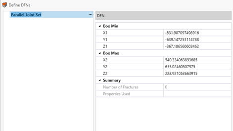
3. Enter the scale of the Box as following
   1. Box Min: X1 = -530, Y1=-640, Z1=-370
   2. Box Max: X2=540, Y2=650, Z2=230
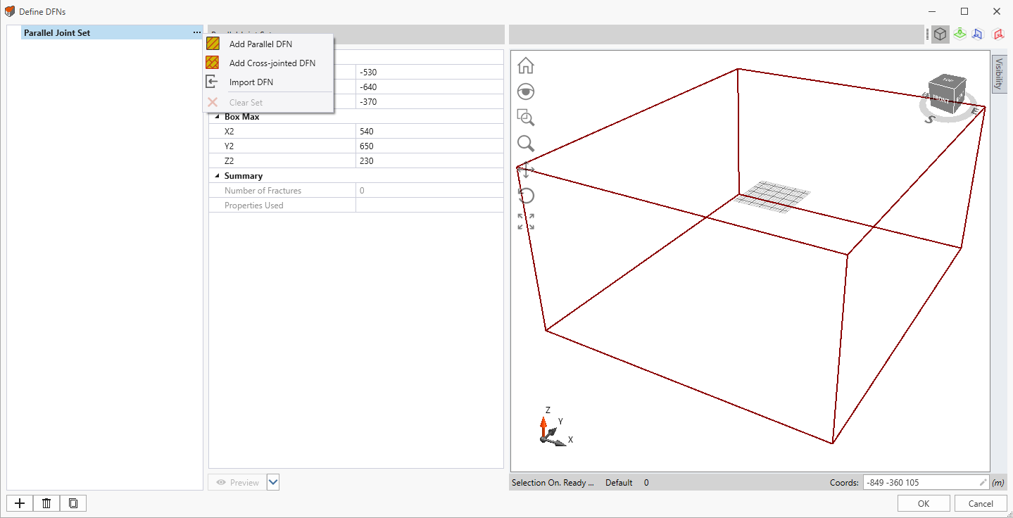
4. Select Add Parallel DFN from the three dots drop down menu next to the DFN to create a new set of parallel joint network.

3.1 JOINT NETWORK INPUT

When new Parallel or Cross jointed DFN is added, the Define DFNs dialog automatically selects the newly added DFN type and the input data fields also switches accordingly.

1. Keep the Property of the DFN to Joint 1 and Infinite Plane enabled.
2. Enable the Is Spacing Stochastic with Normal spacing distribution and specify the following distribution parameters:
• Sp. Mean = 20
• Sp. Std. Dev = 7
• Rel. Min = 10
• Rel. Max = 30
3. Specify the joint orientation of 63/259 for dip/dip direction and click Preview. Then click OK.

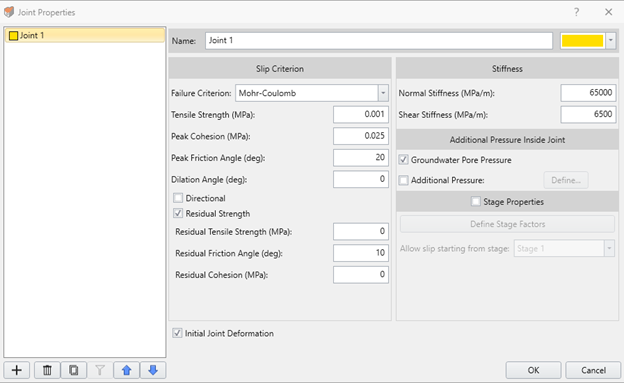
The model should already have joint properties defined, but it can be checked to make sure that the assigned inputs are as shown below

4. Select: Materials > Joints > Define Joint Properties

3.2 ADDING DFN

We are going to assign the DFN to Shale entity.

1. Select the Shale entity from the visibility tree or viewport (But make sure the Entity Selection mode is enabled when selecting from the viewport).
   
2. Select: Materials > Discrete Fracture Networks (DFNs) > Add a DFN…
3. The Add DFN dialog should appear as below (Checking the Preview check box geometry of the joint network). Clicking OK will add DFN to the Shale entity.

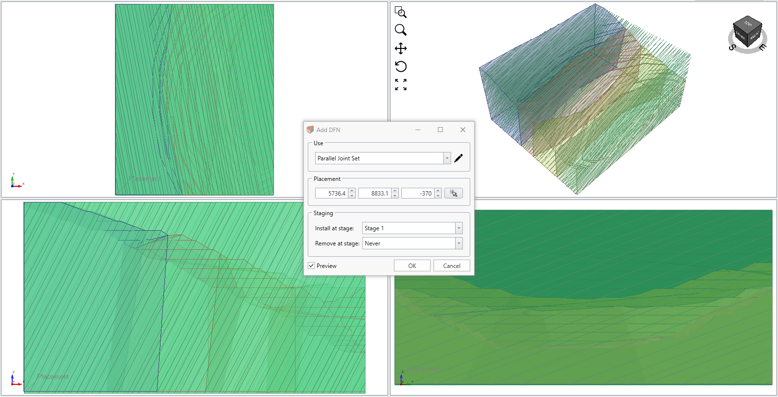
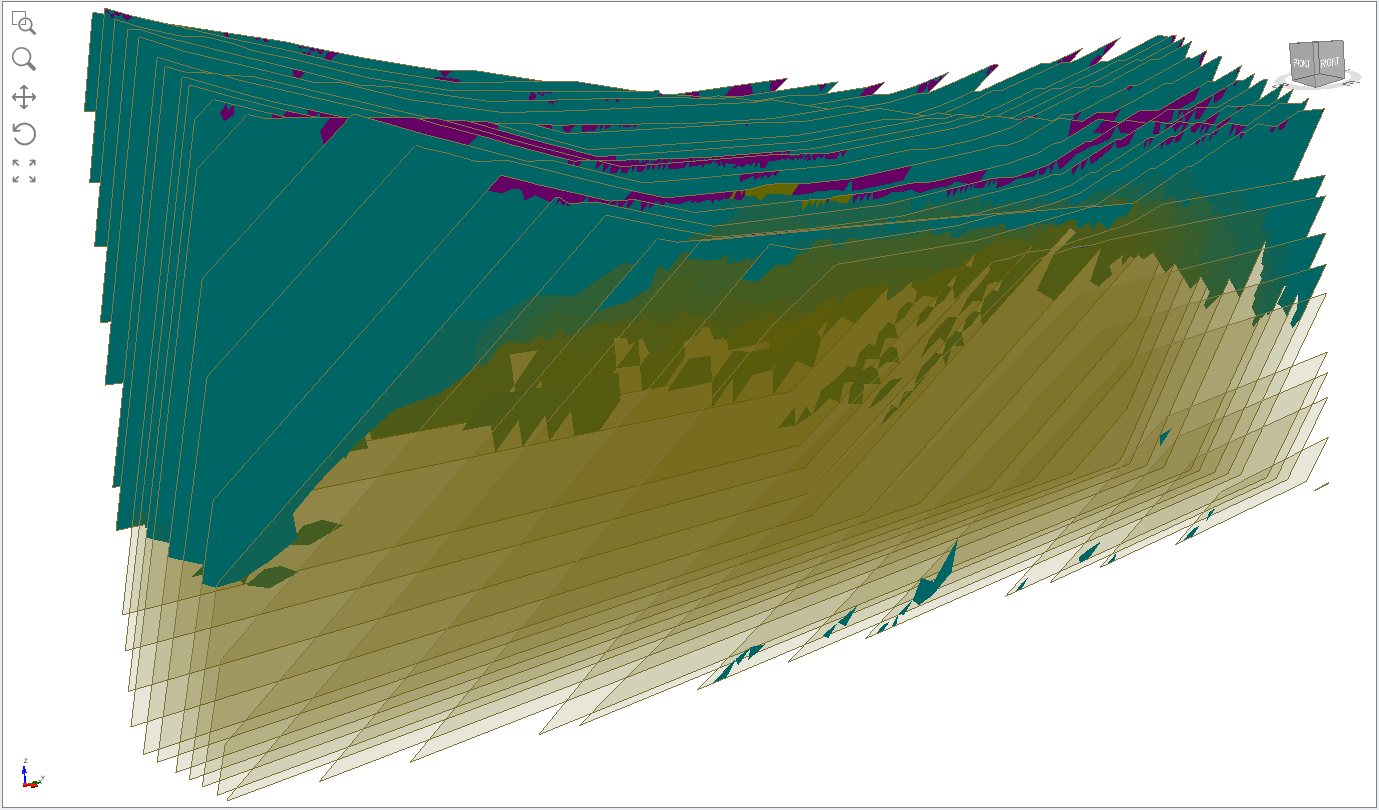
The model with DFN successfully added (and selected) to the Shale entity should look similar to below. As described earlier on note, the joint distribution in the model generated following the described steps may NOT look identical to the figure below.

3.3 DIVIDE ALL GEOMETRY

Now that we have completed assigning DFN, we can use the Divide All Geometry function to fully integrate the DFN for the stress analysis computation.

1. Select: Geometry > 3D Boolean > Divide All Geometry

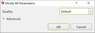
The Divide All Parameters dialog appears, which can be used to fine-tune the details of subdividing external boundaries. Keeping Quality in Default is suitable for a wide range of models in general, however, there are cases where changing the setting is required to successfully intersect every geometry with the external volume.

2. We will keep the Quality default for this tutorial. Select OK to begin dividing.

4.0 Field Stress

1. Select the Loads workflow tab

This tab allows you to define loading condition and field stress.

2. Select: Loading > Field Stress
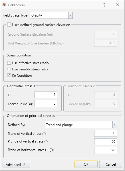
3. The Gravity field stress option is used for this model, which applies in-situ stress field that varies with depth. Gravity field stress is typically used for surface or near surface excavations modelling, which has varying ground profile elevation.


The depth and the unit weight of overlying material determines the vertical stress distribution throughout the model. The horizontal stresses are then calculated by multiplying the vertical stress by the Horizontal/Vertical Stress Ratio(s).

4. Since this model does not consists of soil material, Use effective stress ratio is disabled. In the Field Stress dialog, the following parameters are used to define a Gravity stress field.

5.0 Restraints

1. Move to the Restraints workflow tab to assign restraints to the external boundary of the model .

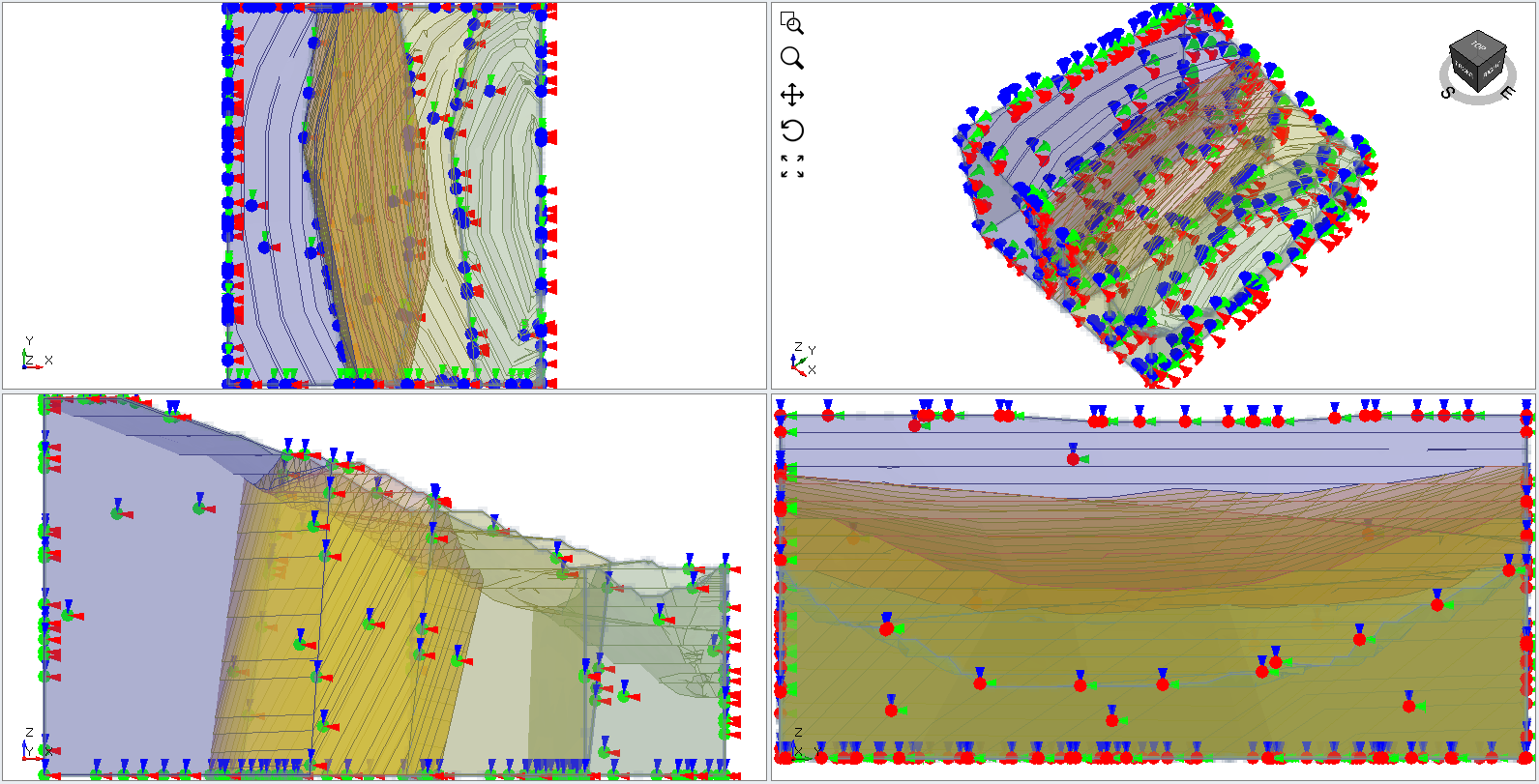
For this tutorial, we need to apply XYZ restraints on all surfaces other than the excavated slope face.

2. Select: Restraints > Auto Restrain (Surface)

After the application of restraints, your model should look similar to the one below

6.0 Mesh

1. Next, we move to the Mesh workflow tab

Here, we may specify the mesh type and discretization density for our model. For this tutorial, we will use a default setting, 4-noded tetrahedra graded mesh.

1. Select: Mesh > Mesh Settings
   
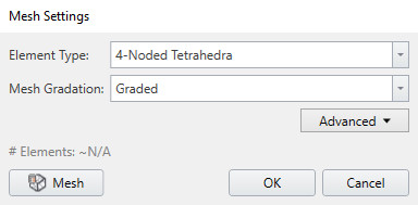
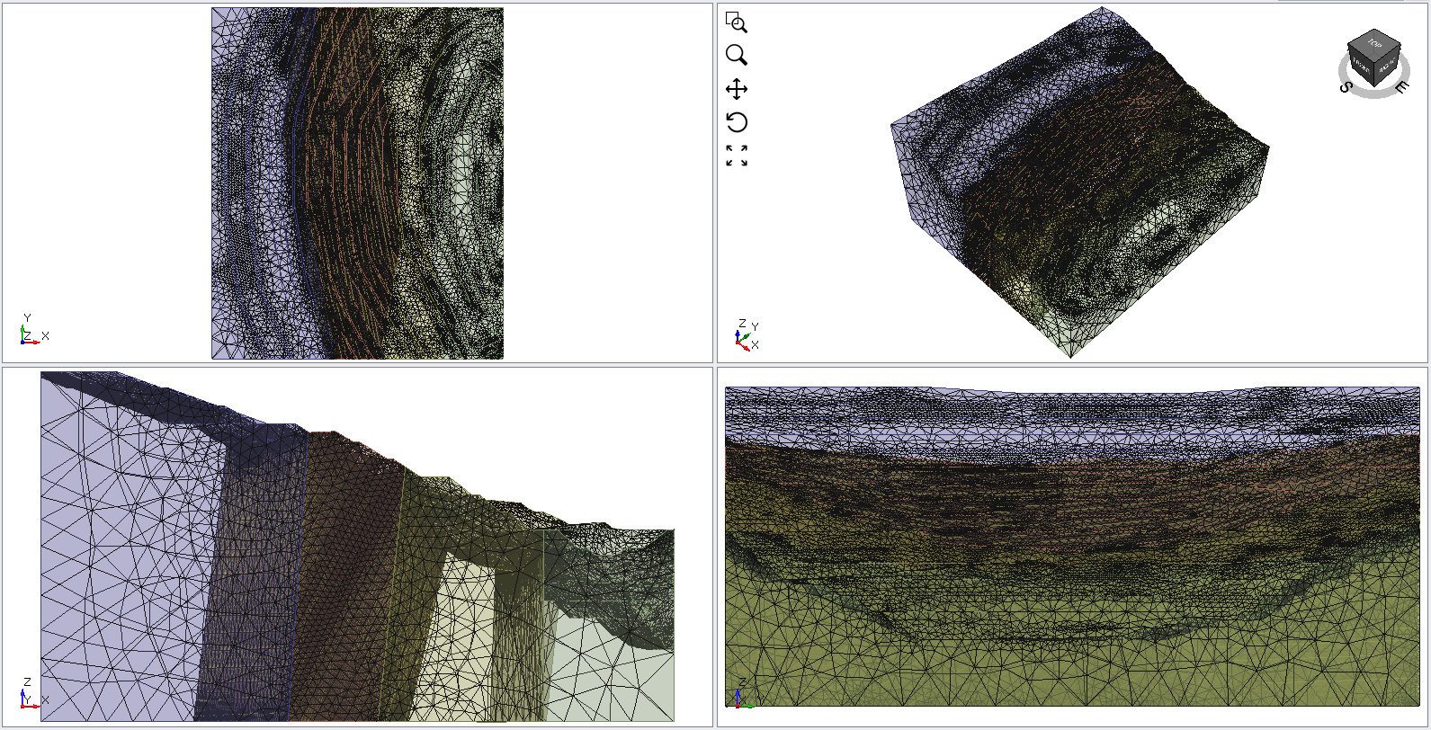
2. Click the Mesh button from the dialog to begin meshing the model and click OK when completed.

Your model should look like the figure below.

7.0 Computing Results

1. Next, we move to Compute workflow tab

From this tab, we can compute the results of our model. Before commencing the stress analysis computation, it is recommended to save the final model as a separate file so that you can access the original file anytime: File > Save As.

2. Select: Compute > Compute

8.0 Result Interpretation

1. Next we move to Results workflow tab

8.1 SOLID DEFORMATION

Following procedures will guide you to see the deformation of solid elements.

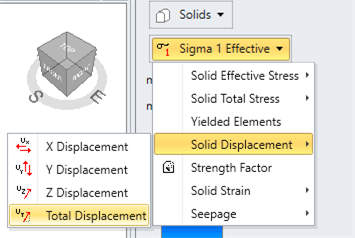
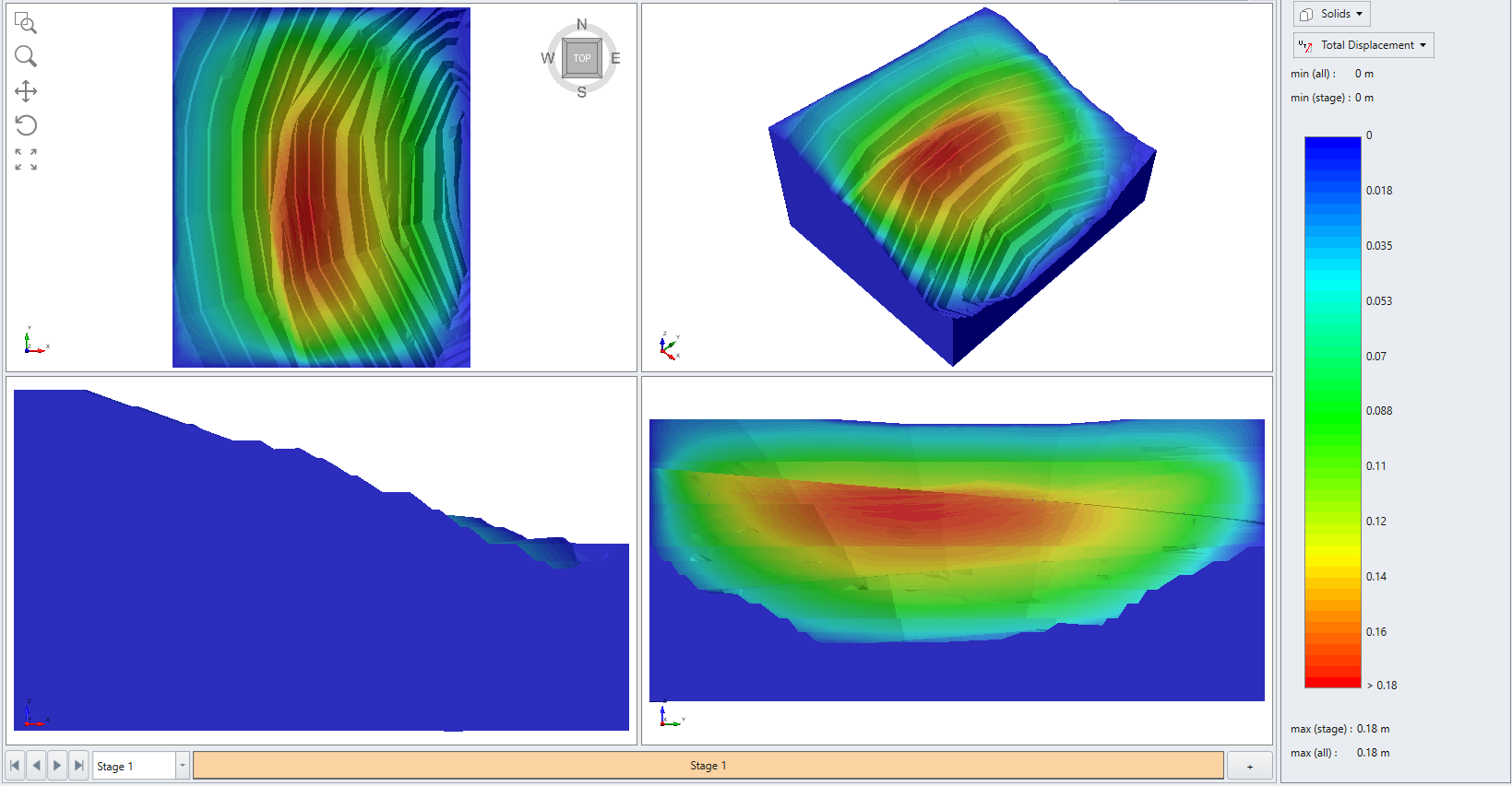
1. Select Solid Displacement > Total displacement for the contour plot.
   
2. Select: Interpret > Show Exterior Contour

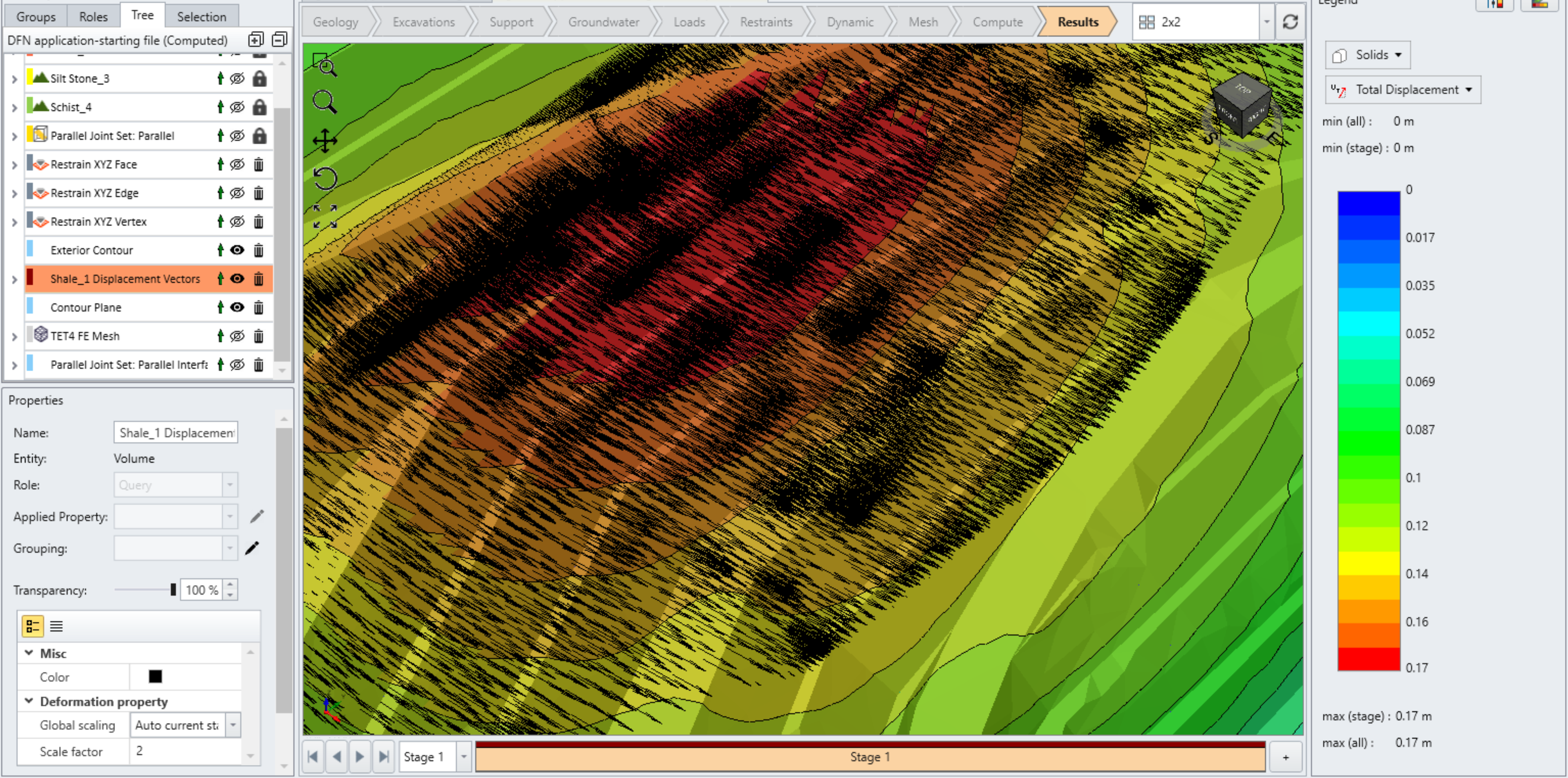
The slope deformation is concentrated at the upper region of the shale with the maximum total displacement of 0.18 m.

3. Having Shale entity selected, select Interpret > Displacement Vectors
4. The vectors that show the direction of the element displacement appears. Since the size of these vectors are too small to visualize, having the newly created Displacement Vectors entity selected from the visibility tree, increase the Max Length to 20 under Properties pane. Also, switching the vector color to black produce vectors more distinct like the figure below.

To examine the displacement within the region of high deformation with respect to depth, we will create a contour plane to make a section view of the contour.

5. Select: Interpret > Show data on plane > XZ Plane
6. Enter the origin location/orientation of the plane as following:
   1. X1 = 12536.7, Y1= 18814.9, Z1= -69.1
   2. Orientation (Dip/Dip Direction): 90/-9.0
7. Click Add and then Close.
   
8. Hide all entities other than the created contour plane and maximize the Front view by right clicking on the viewport box in the top right hand corner.
   
9. The contour plane shows discontinuous displacement due to shearing of joints (See Section 8.2 for the state of the joint). The modeling result indicates that this region is prone to toppling failure. Toppling effect becomes more conspicuous after reducing the Interval Count to 20 and with Show Contour Lines enabled from Contour Options
   
10. Click OK.
    

8.2 JOINT STATE

The state of joint elements can be examined by following the procedure:

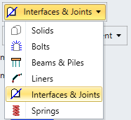
1. Switch the Results Element Type under Legend from Solids to Interfaces & Joints

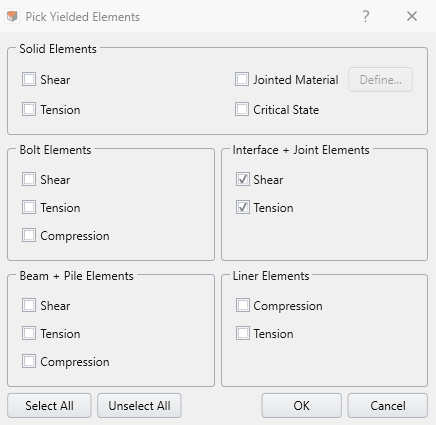
2. Select: Interpret > Yielded Elements > Pick Yielded Elements. From the Pick Yielded Elements dialog, enable Shear and Tension under Interface + Joint Elements.
   

3. Click OK. The yielded elements (shear and tension) will be displayed. But, since the contour data already is active, yielded joint elements may not be clearly visible. Following additional steps show tricks to help to visualize the yielded elements, which can be done by hiding the projected contour data. We can change the contour legend to be out of the range. If no changes were made to the contour data type, it should be set to Relative X Displacement in default (and the following steps are explained assuming that the Relative X Displacement plot is displayed).
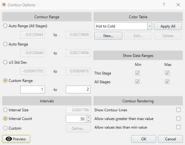
4. Select: Interpret > Contour Legend > Contour Options
5. Switch Contour Range from Auto Range to Custom Range (1 to 2).

The view port should show the location of failed joint elements as below. The modeling result shows the shear failure of most of the joint elements at the upper region of the shale, where the maximum deformation happens.

This concludes the tutorial.