Transient Dam

1.0 Introduction

This tutorial demonstrates some of the transient groundwater features of RS3. Here we create a dam with a changing head to examine the pressure head with time.

All tutorial files installed with RS3 can be accessed by selecting File > Recent > Tutorials folder from the RS3 main menu. The starting file of this tutorial can be found in the Transient Dam - starting file.rs3v3 file and the finished product of this tutorial can be found in the Transient Dam.rs3v3 file.

2.0 Starting the Model

1. Select File > Recent > Tutorials Folder.
2. Open the starting file Transient Dam - starting file.rs3v3
3. Select: File > Save As to save a copy of the project.

The model should have initial project settings already defined for the user. Go to the Project Settings to check the initial inputs:

1. Select: Analysis > Project Settings

The Project Settings dialog is used to configure the main analysis parameters for your RS3 model.



2. Select the [Groundwater] tab.
   
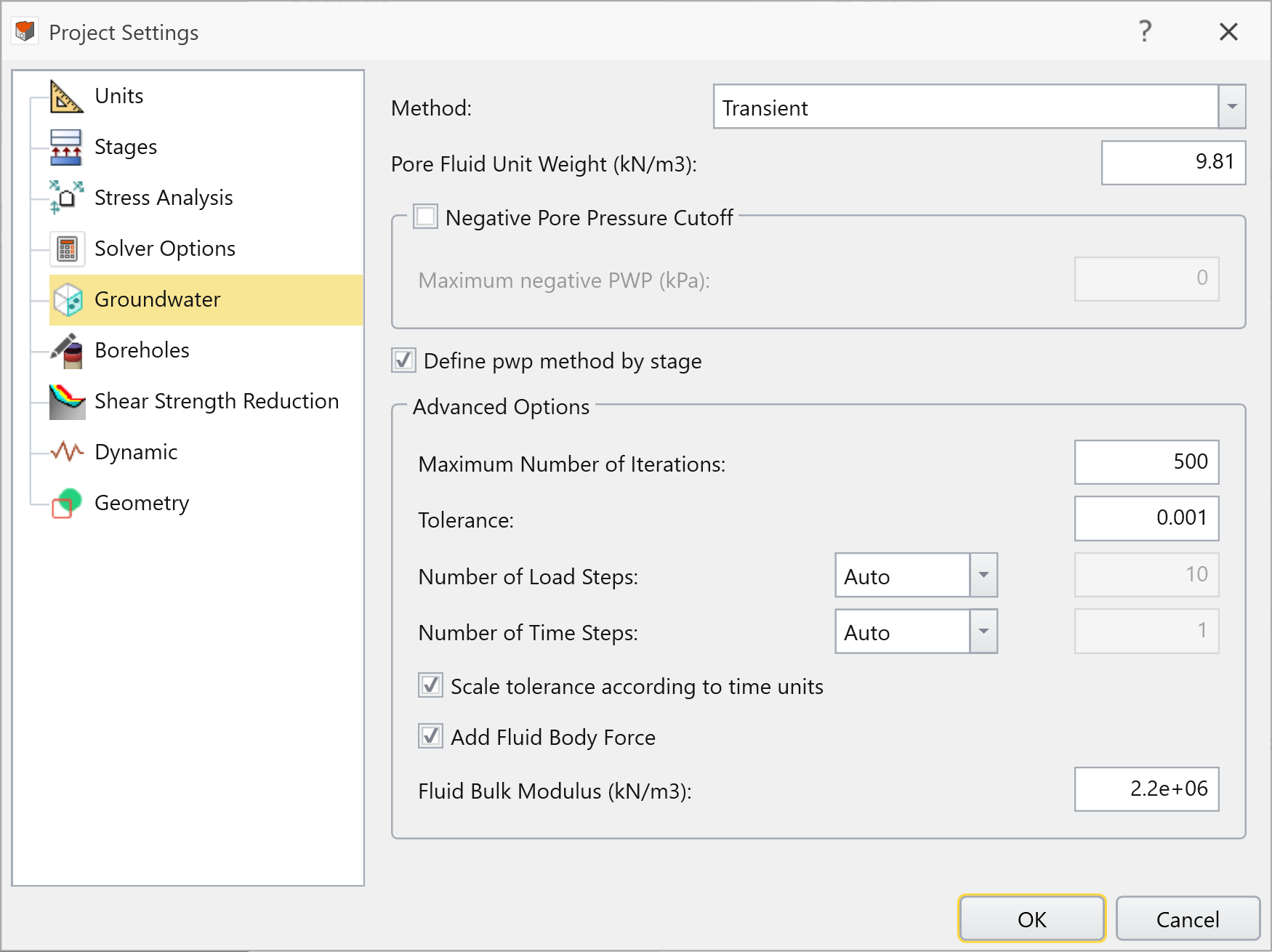
3. Check that Method = Transient, and make sure Define pwp method by stage = activated.
   
4. Select the [Stages] tab.
5. Check that Number of Stages = 6, and for Stages 2-6 the PWP method = Transient with time = 2, 4, 6, 10, 50 (also see below).
   
6. Click OK to close the dialog.

3.0 Defining the Materials

Under the same workflow tab (Geology or Excavations) you can assign the materials and properties of the model through materials setting.

The model should have the materials already defined for the user. Please check the following inputs:

1. Select: Materials > Define Materials.
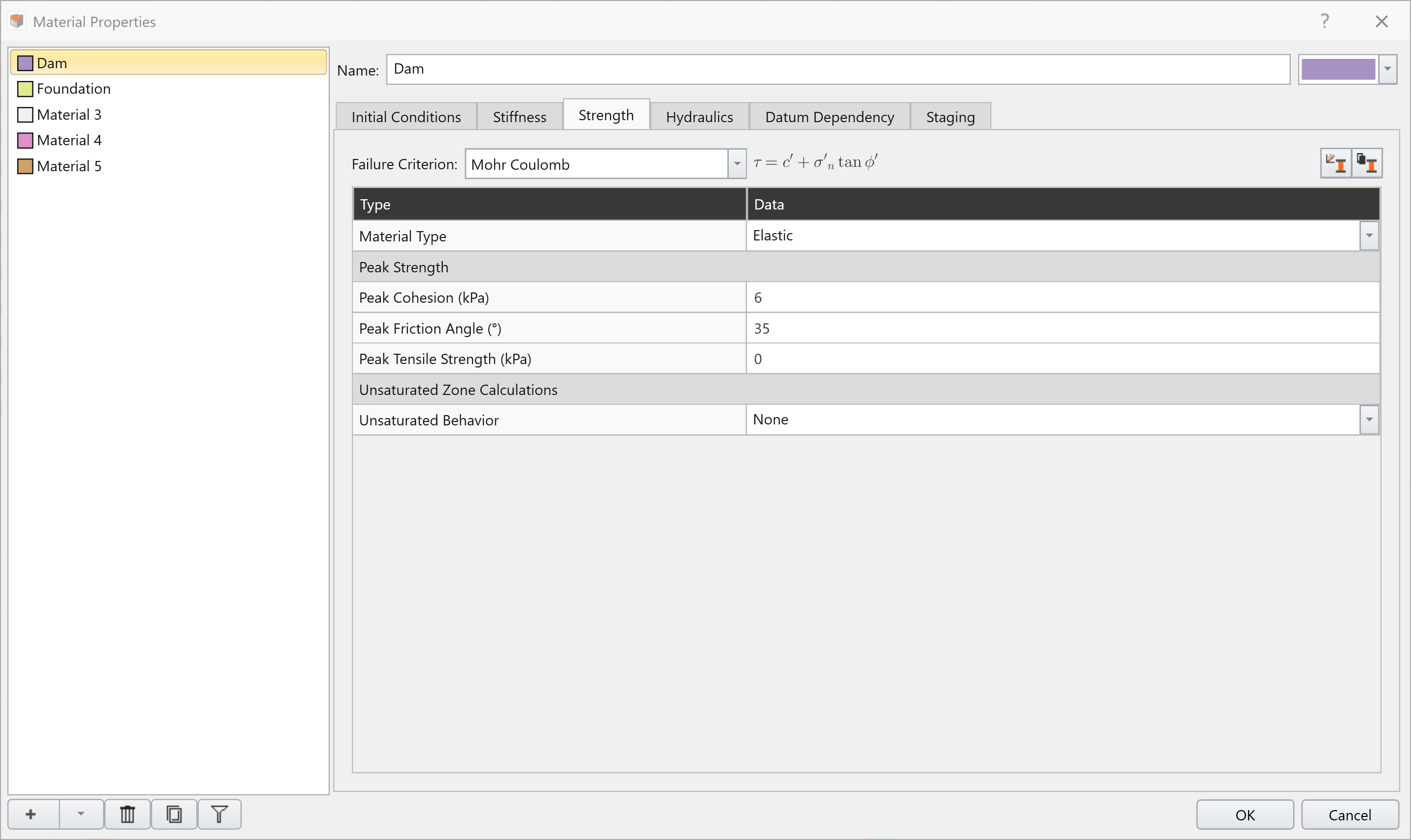
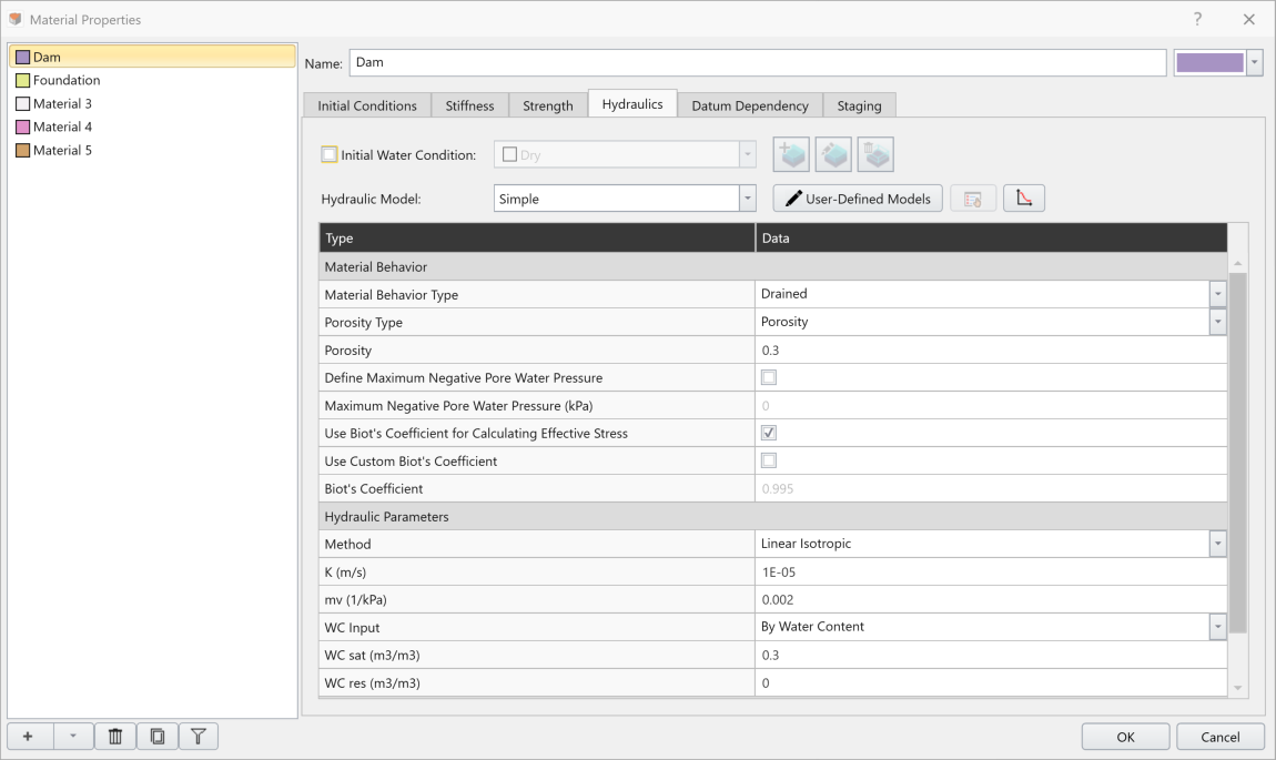
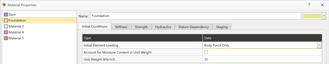
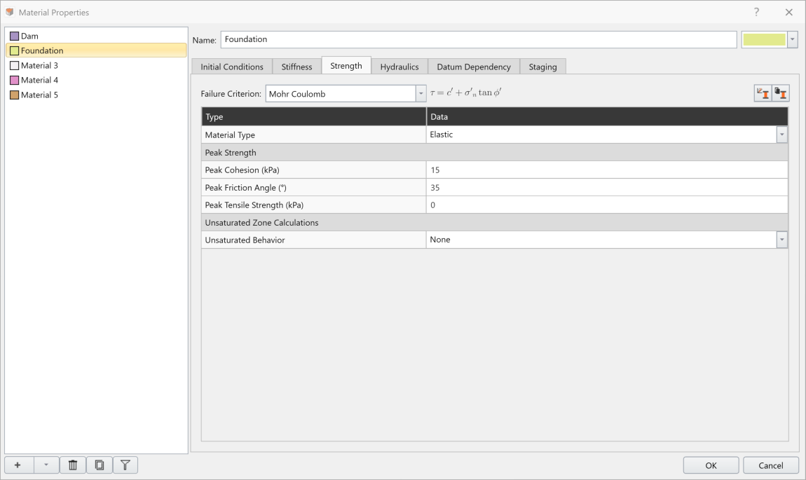
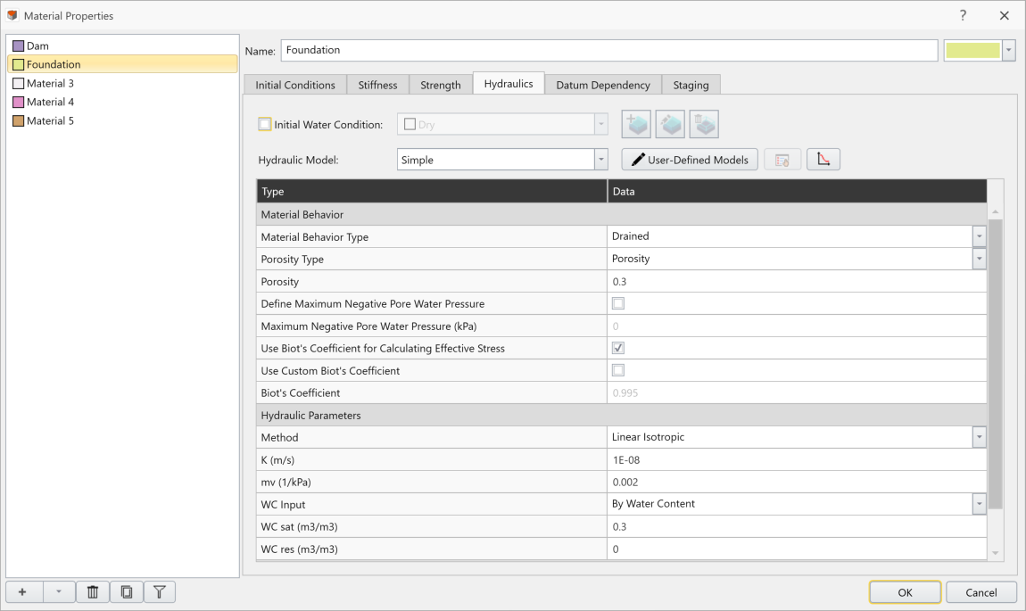
2. In the [Strength] and [Hydraulics] tab respectively, check the strength parameters and hydraulics parameters.

Material 1 - [Strength]:

Material 1 - [Hydraulics]:

Material 2 - [Initial Conditions]:

Material 2 - [Strength]:

Material 2- [Hydraulics]:

1. Click OK to close the dialog.

4.0 Creating Geometry

1. Ensure the Geology workflow tabis selected from the workflow at the top of the screen.

4.1 CREATING THE DAM PROFILE

1. Select: Geometry > Polyline Tools > Draw Polyline
   On the left of the screen, a Draw Polyline dialog will open.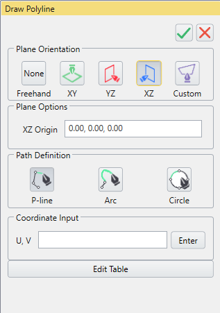
   
2. Select Plane Orientation = XZ
3. Then enter the following U, V Coordinates (press [Enter] between each pair):
   • (0, 0)
   • (100, 0)
     
   • (100, 10)
     
   • (75, 10)
     
   • (51, 22)
     
   • (44, 22)
     
   • (20, 10)
     
   • (0, 10)
     
   • (0, 0)
     
4. Select the green checkmarkto finish the polyline.
5. Select the “PolyLine” entity in the visibility pane.
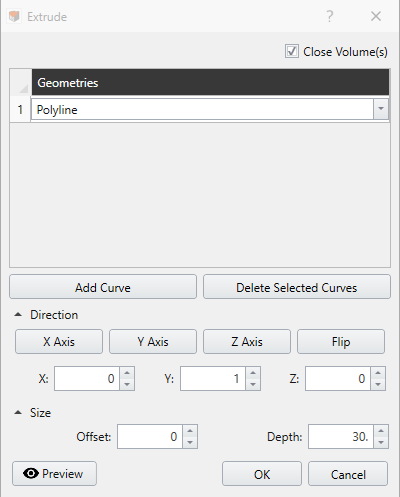
6. Select: Geometry > Extrude/Sweep/Loft Tools > Extrude or select Extrudeicon in the toolbar.
7. Enter Direction (x, y, z) = (0, 1, 0), Depth = 30, and click preview to see the geometry. Select OK.
   
8. Select the "Polyline_extruded” entity in the visibility pane.
9. Select Geometry > Set as External in the menu.
   

4.2 SEPARATING THE DAM LAYERS

In this model, we will have a foundation with a different dam material on top. We need to draw the line that will be used to separate the materials.

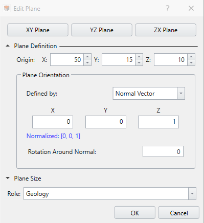
1. Select: Geometry > 3D Primitive Geometry > Plane
2. Select Plane Definition = XY Plane.
3. Under the Plane Definition set:
   
   1. Plane Origin (x, y, z) = (50, 15, 10),
      
   2. Plane Normal (x, y, z) = (0, 0, 1).
      
   3. Leave Rotation Around Normal = 0,
      
4. Click OK.



Next, we need to create two closed shapes from the plane:

5. Select: Geometry > 3D Boolean > Divide All Geometry
   
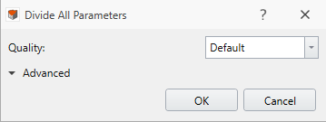
6. Click OK.


After doing so, you’ll find there are two volumes, one defining the top dam, the second the base.

7. Select the top volume from the visibility pane. In the Properties Pane, select Applied Property = Dam, and change the Name to Dam.
8. Select the bottom volume from the visibility pane. In the Properties Pane, select Applied Property = Foundation, and change the Name to Foundation.

5.0 Defining Groundwater

5.1 STEADY-STATE GROUNDWATER BOUNDARY CONDITIONS

1. Select the Groundwater workflow tab
   

We will now define the groundwater boundary conditions.

1. Make sure that Stage 1 is selected in the bottom stage tabs, then select Faces Selectionin the toolbar.
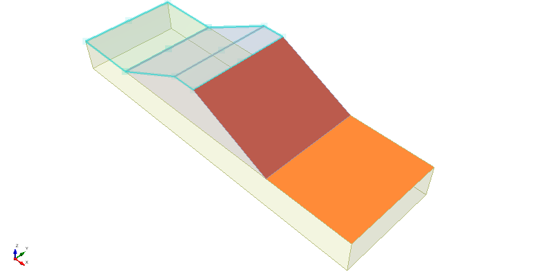
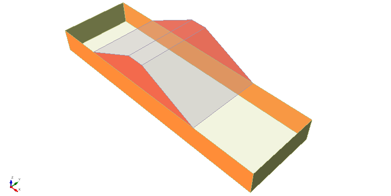
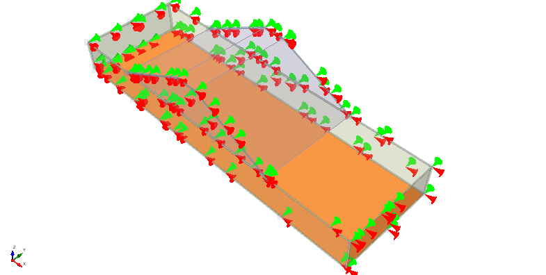
2. While holding down the [Ctrl] key, select the faces highlighted in the following image in order to apply groundwater boundary conditions (Top two surfaces of the dam, and top surface of the foundation):
   
   
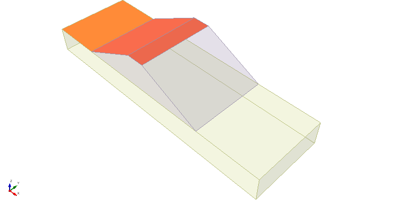
3. Select: Groundwater > Add Groundwater Boundary Conditions
   
4. Select the pencil iconbeside the drop down to edit the groundwater boundary conditions to open the Groundwater Properties dialog.
   
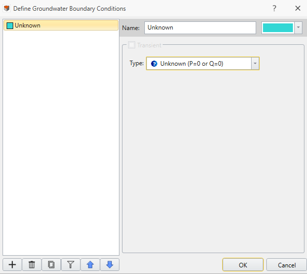
5. Enter Name = Unknown, Type = Unknown (P=0 or Q=0), then select OK, then OK to add the BC, ensuring it is installed at Stage 1 and never removed.
6. While holding down the [Ctrl] key, select the faces highlighted in the following image (other two top sides of the model)
   
7. Select: Groundwater > Add Groundwater Boundary Conditions
8. Select the pencil iconbeside the drop down to edit the groundwater boundary conditions to open the Groundwater Properties dialog
9. Add a new groundwater boundary condition by pressing the add symbol (+) in the bottom right of the dialog.
   
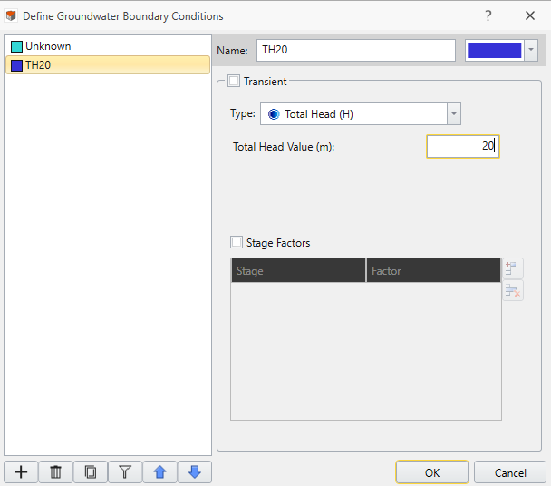
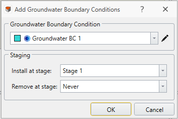
10. Enter Name = TH20, Type = Total Head (H), Total Head Value = 20, then press OK to return to the Add GWBC dialog.
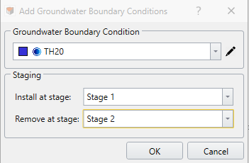
11. For the first stage, the PWP method is steady-state so we will simply add a total head to be removed at Stage 2, then select OK.

5.1.1 Transient Groundwater Boundary Condition

1. Select the Stage 2 tab at the bottom of the RS3 window.
2. Select Faces Selectionin the toolbar.
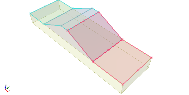
3. While holding down the [Ctrl] key, select the faces highlighted in the following image in order to apply groundwater boundary conditions.
   
4. Select: Groundwater > Add Groundwater Boundary Conditions
5. Select the pencil iconbeside the drop down to edit the groundwater boundary conditions to open the Groundwater Properties dialog.
6. We need to create a whole new transient groundwater property, add a new groundwater boundary condition by pressing the add symbol in the bottom right of the dialog. Set it up as shown and press OK.
   
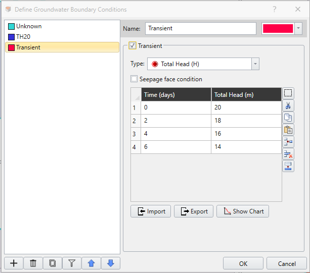
7. Enter Name = Transient, select Transient, Type = Total Head (H), type in Time = (0, 2, 4, 6), and Total Head = (20, 18, 16, 14), then select OK to return to the Add GWBC dialog.
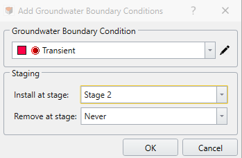
8. We want to apply the transient condition at Stage 2 [Install at Stage Condition to Enter] until the end of analysis. Once the settings match the screenshot below, then select OK.

6.0 Adding Field Stress

1. Next, we go to the Loads workflow tab. This tab allows you to edit the loading conditions.
2. Select: Loading > Field Stress
3. Leave Settings as default. Field Stress Type is set to Gravity. Click OK.

7.0 Setting Boundary Conditions

7.1 ADDING MODEL RESTRAINS

1. Move to the Restraints workflow tabto assign restraints to the external boundary of the model.

RS3 has a built in “Auto Restrain” tool for use on underground models but we can’t utilize for this tutorial because of the inclined free surface.

1. For custom restrain definition, select the following faces in the model (using Face Selectionin the toolbar):
   
2. Select: Restraints > Add Restraints/Displacements > Restrain XY, then press OK.
3. Next, we will select the bottom face to restrain.
   
4. Select: Restraints > Add Restraints/Displacements > Restrain XYZ, then click OK.

8.0 Meshing

8.1 CONFIGURING AND CALCULATING MESH

1. Next, we move to the Mesh workflow tab. Here we may specify the mesh type and discretization density for our model.
2. Select: Mesh > Mesh Settings
3. Use the default options:
   1. Element Type = 4-Noded Tetrahedra, Mesh Gradation = Graded.
4. Select Meshto mesh the model.
   
   
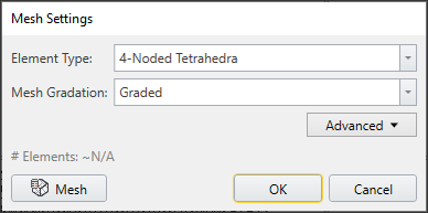
5. Click OK.
   

9.0 Computing Results

1. Next, we move to Compute workflow tab
   
2. From this tab, we can compute the results of our model. First, save your model: File > Save As.
3. Next, you need to save the compute file: File > Save Compute File. You are now ready to compute the results.
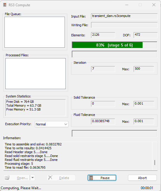
4. Select: Compute > Compute Groundwater Only
   

10.0 Interpreting Results

10.1 DISPLAYING THE RESULTS

1. Next, we move to Results workflow tab. From this tab, we can analyze the results of our model. First, refresh the results:
2. Select: Interpret > Refresh All Results
   

Refreshing the result allows us to plot new results of the model. Although we did not have any previous results from this model, it is good practice to refresh results before we view new contour plots.

On the top right corner of the Results tab, you should see two drop down menus in the Legend:

1. Ensure [Solids] is selected from the Element drop down menu.

We will analyze a number of different “Data Type” results. Let’s turn on the exterior contours so we can see some results:

1. Select: Interpret > Show Exterior Contour

Under any non-groundwater calculations, the exterior contour will not appear, as only groundwater results were computed

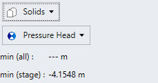
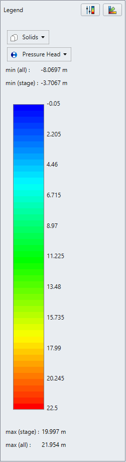
Pressure Head

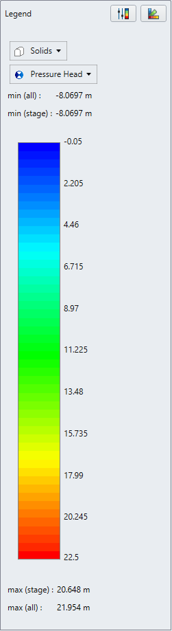
1. In the Legend, change data type Seepage > Pressure Head
   
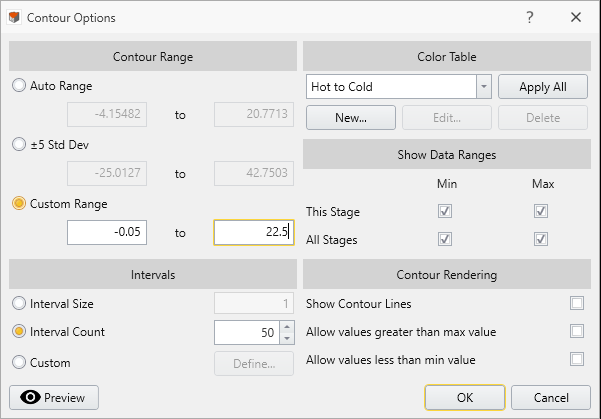
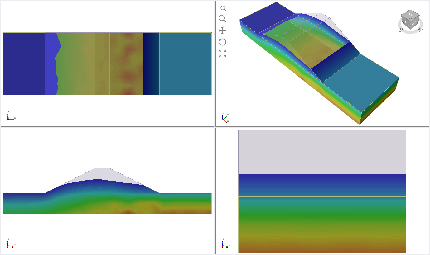
2. Select Interpret > Contour Legend > Contour Options Set the Custom Range = -0.05 to 22.5, then click OK.

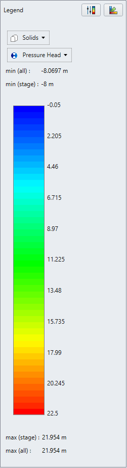
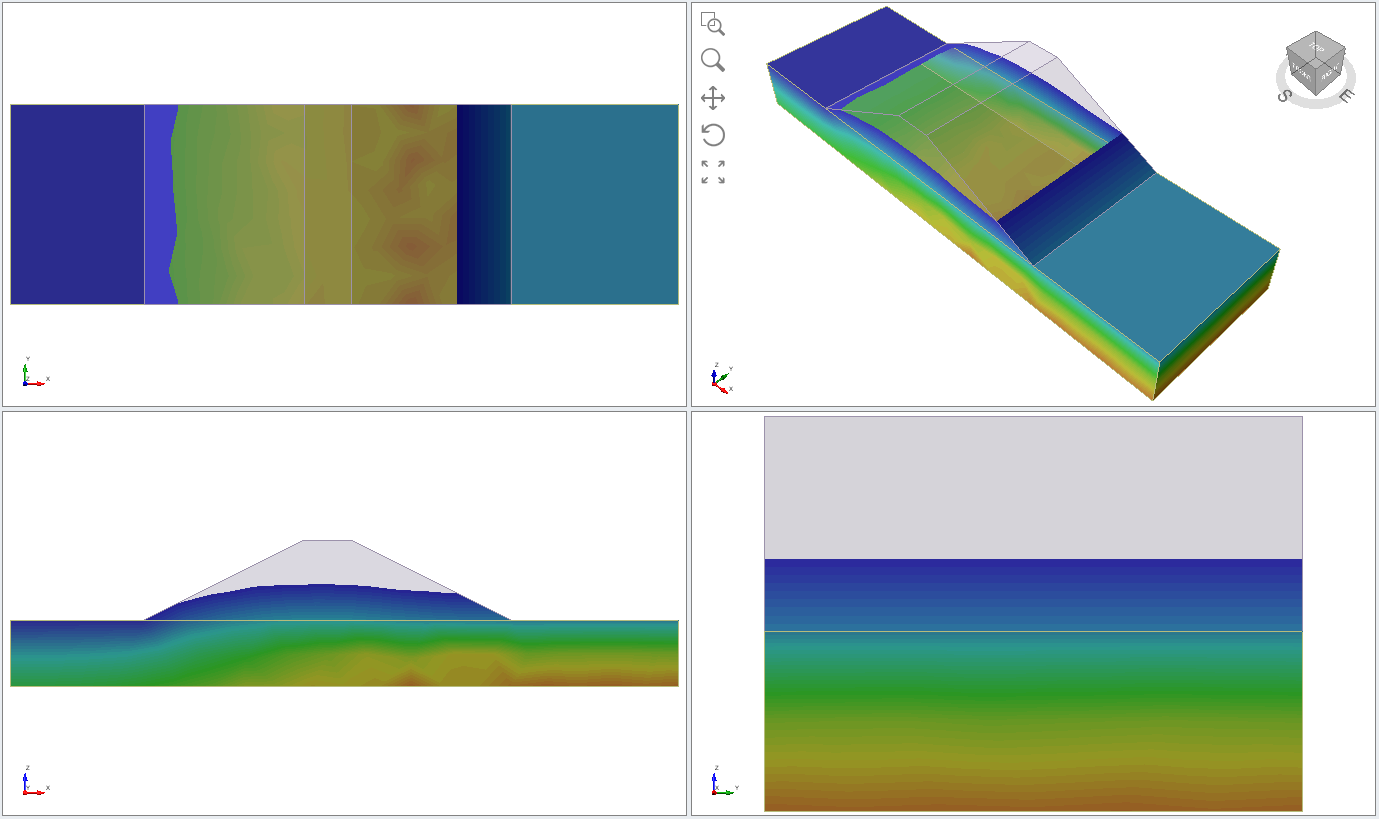
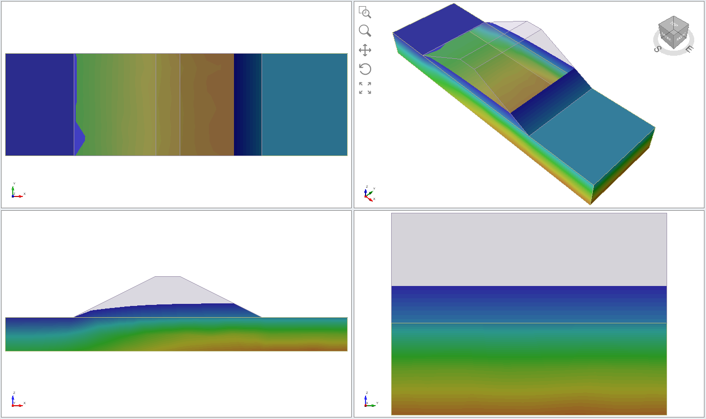
The pressure head results at Stage 1, 2, 3, 4, 5, and 6 are shown below respectively

Stage 1
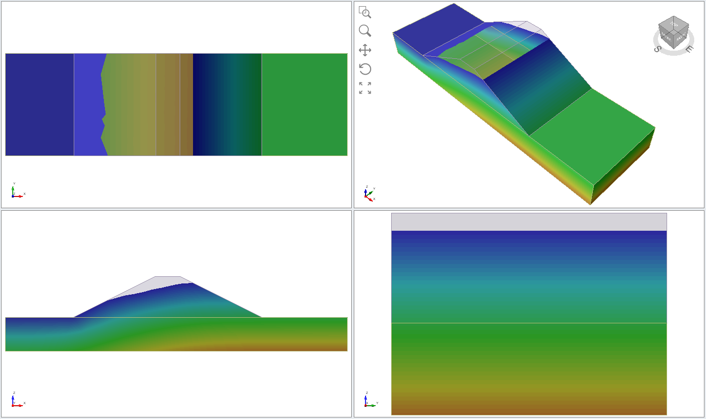Stage 2
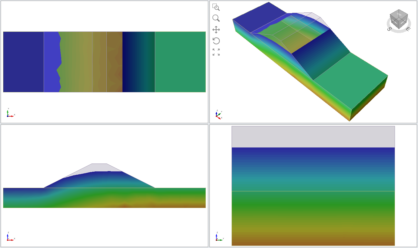Stage 3
Stage 4
Stage 5
Stage 6

Other results such as total and excess pore pressure are available to view. This concludes the tutorial.