Dips Knowledge Base

The following questions are common modelling-related tech support questions:

Can I convert alpha/beta from an oriented core drilling into dip/dip direction or strike/dip data?

Yes, Dips can convert alpha-beta measurements from oriented cores into true dip/dip direction data using the Borehole Traverse option.

Please see the following sections from the Dips Online Help for more information:

• Overview of Traverses
• Traverse Orientation Borehole
• Borehole Orientation Data Pairs
• Dips Tutorial 11 - Oriented Core and Rock Mass Classification
• Additional Dips Tutorials

Note that once you have entered the alpha-beta and borehole Traverse information into Dips you can output the data in dip/dip direction or strike/dip format using the Save Processed File option.

How can I correct the bias of televiewer data (dip and dip direction) in Dips?

If the borehole fracture data is already processed into true dip/dip direction (e.g. from optical or acoustic televiewer) then you simply define a linear Traverse where the Orient1/Orient2 values in the Traverse dialog are equal to the Trend/Plunge of the borehole. Note: for a linear Traverse the Orient1/Orient2 values in the Traverse dialog are always in Trend/Plunge format (regardless of the Global Orientation format of the joint measurements).

The Terzaghi weighting (bias correction) for a linear Traverse is the same as a borehole Traverse (oriented core) i.e. a borehole Traverse is equivalent to a linear Traverse for the purpose of bias correction. You can verify this by taking an oriented core (borehole file), saving a processed version of the file with the Save Processed option in the File menu, and then re-defining a linear Traverse for the data and comparing weighted results.

For wedges sliding on one plane, can I use Dips to determine which joint is the sliding joint?

This information is not directly available in Dips. For wedges sliding on one plane, Dips does not identify which is the sliding plane and which is the release plane.

However, follow the instructions below for a way to determine this information:

Select File>Export>Export Data to Excel, and all available analysis data will be exported to an Excel file.

Select the Plane Intersections tab. This lists analysis data for the Direct Toppling and Wedge Sliding modes.

In the Wedge Sliding column, you will see a flag which identifies critical intersections (P2=sliding on two planes, P1=sliding on one plane)

The associated planes from the original Dips file are identified in the columns Plane ID#1 and Plane ID#2. This gives the row ID number of the planes from the original Dips file.

You can go back to the original file and get the dip/dip direction of the two planes forming the wedge.

If you have SWedge you can simply input these two planes into SWedge, along with the slope orientation. The SWedge Info Viewer will give you the details about sliding plane / release plane. For more information about SWedge see the SWedge product page.

You can also determine the Wedge Sliding mode graphically on a stereonet. The following article is useful:

Yoon, W.S., Jeong, U.J., and Kim, J.H. (2002) Kinematic Analysis for sliding failure of multi-faced rock slopes. Engineering Geology. 67:51-61

How can I calculate the apparent dip of a plane from another orientation in Dips?

To calculate the apparent dip of a plane, add the plane to the stereonet using the Add Plane option. Then use the Add Line option in the Tools menu to add a line at the desired orientation. The intersection of the great circle and the line will give you the apparent dip, which you can measure graphically. To get the coordinates, hover the mouse over the intersection point, and make sure that the Convention option for coordinate (click on the box in the lower right corner of the stereonet) is set to Trend/Plunge, so that the coordinates of the intersection line are displayed in Trend/Plunge format.

How do I plot Great Circles in Dips?

To display all great circles for all of the poles in the main Dips spreadsheet, use the Grid Data Planes checkbox in the Sidebar plot options (Plot Options > Planes > Grid Data Planes).

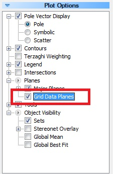
When you add an individual plane (Planes > Add User Plane option), you can display the great circle when you initially add the plane (plane visibility checkbox in the dialog) or after you have added the plane, with the Edit Planes option.

To quickly toggle the display of all user planes and/or mean planes from sets, use the Plot Options > Planes > Major Planes check boxes.

Why am I seeing the message "Too Many Entries for Grid Intersections?"

There is a hardcoded limit of 8000 poles, which generates the intersection message you are seeing. The number of intersections is proportional to the number of poles squared (n*(n-1)/2), so 4000 poles generates 32 million intersections. As Dips is a 64-bit program, memory usage is limited, so we had to put a limit on the number of intersections that are calculated.

For now, the only way around this is to reduce or filter your data below 8000 poles in order to compute intersections.

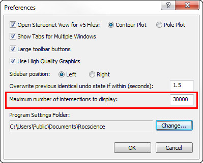
There is another option in the Preferences dialog ( File > Preferences) which allows you to control the number of intersections which are displayed. The default is 30,000. This is to prevent the entire stereonet from getting obscured by the intersection points, which tends to happen with large files. However, this option is independent of the 8000 pole limit, which cannot be user defined.

Why is there a limit of 30,000 intersections in the preferences dialog?

With large data files you end up with millions of intersections, which grinds the plotting to a halt. An arbitrary default limit of 30,000 is set in the Preferences dialog in the File menu. You can increase this number as required, but the display and plotting of intersections may take a very long time, and you may also run into memory limitations on your computer.

If n=number of poles, then the number of possible intersections is given by:

n*(n-1)/2

See the Intersections Overview topic in the online help for more information.

Keep in mind that the limit in the Preferences dialog refers to intersections (not poles), and the limit is a display option (i.e. if the number of intersections exceeds this limit, then the intersections will NOT be plotted or contoured). Calculations involving intersections (such as Kinematic Analysis of Wedge Sliding) will still be carried out.

Can coordinates be entered into Dips?

Dips does not have any capability to plot joint locations in x,y,z coordinates (in either 2D or 3D).

You could enter x,y,z coordinate data into the spreadsheet using extra columns, but you would only be able to plot the information on the stereonet (symbolic pole plot) or using histograms/chart plotting, which is of limited usefulness.

What is the difference between the Global Mean and the Global Best Fit?

The Global Best Fit is a best-fit plane through the pole vectors. This results in a plane which is approximately parallel to the pole vectors, whereas a mean plane is approximately perpendicular to the pole vectors. A best-fit plane is typically used for fold analysis, where it is of interest to find a plane which is perpendicular to a fold axis (and therefore parallel to the pole vectors of the folded planes). You can see this if you use the Fold Analysis option in the Tools menu, select a group of poles with the freehand window, and you will notice that the best fit great circle passes through the selected poles.

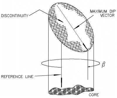
Article on orientation of borehole data

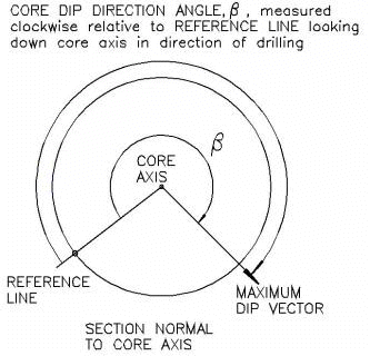
Discontinuity measurements on oriented cores are in terms of alpha and beta angles measured with respect to the core axis. The beta angle is measured with respect to a reference line scribed along the length of the core. The position of this reference line is measured with respect to the TOP of the core.

For example:

• if the reference line is coincident with the TOP of the core, then Orientation 1 = 0
• if the reference line is at the bottom of the core, then Orientation 1 = 180

Typically, the reference line is either at the top or the bottom of the core, so Orientation 1 = 0 or 180.

However, Dips allows for a general definition of the position of the reference line, so Orientation 1 can be any angle between 0 and 359.

Also, note that the direction of drilling must also be accounted for. As stated in the Online Help, Orientation 1 is defined as:

The angle from the top of the core to the reference line (measured clockwise looking in the down-core direction). Use 0 if the borehole is vertical.

To summarize:

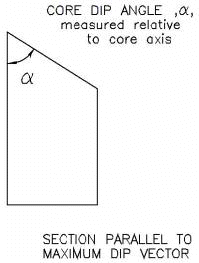
• the alpha and beta angles of discontinuities are measured with respect to the core itself
• Dips then uses the Orientation 1, 2, and 3 values of the borehole to convert the local alpha and beta angles into true dip and dip direction

In order to process your data correctly, you will have to enter all of the data in the exact format required by Dips. If you have used slightly different conventions for any of the measurements, make sure that they are converted to the format described in the Dips Online Help.

Descriptions of Orientations:

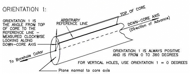
Orientation 1:

For a non-vertical borehole, the TOP of the core is a line along the topmost point of the core, as it was in situ. You need this line in order to relate the orientation of the core to the borehole. For a vertical borehole, there is no "top" of the core, since the hole is vertical. In this case, you can simply enter zero for Orientation 1, and the Orientation 3 value then serves two purposes:

1. To define the position of the core within the borehole, and
2. The direction of north.

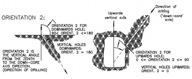
Orientation 2:

Inclination of the borehole axis from the zenith. For example, if the borehole is drilled 20 degrees from vertical, Orientation 2 = 160.

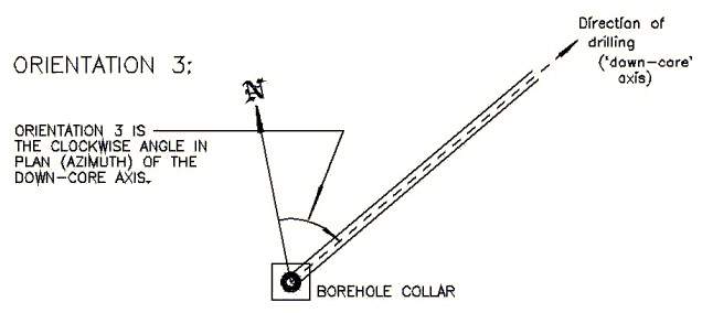
Orientation 3:

This is the direction of drilling with respect to north.

Why is the lateral limit (Kinematic Analysis planar failure) in Dips straight instead of curved (following the contours)?

The straight line lateral limits were chosen partly for simplicity, since the lateral limit is constant regardless of the dip of the slope or failure plane. With the curved lateral limits (defined by a cone) the limits are a function of the dip of the slope.

Both methods are in use and it seems that straight line limits have become more commonly used. The critical area for both approaches is very similar and under most circumstances the number of critical poles will be nearly identical. The reason for imposing lateral limits is due to the observation that planar (and toppling) failure tends to occur when the dip direction of the failure plane is within a certain angular range of the slope dip direction. This limit is empirical and values between plus/minus 15 and 30 degrees have been proposed (e.g. Goodman, Hudson, and Harrison). The kinematic analysis module in Dips is heavily based on Chapter 18 of “Engineering Rock Mechanics” by John Hudson and John Harrison. The book outlines an approach based on linear lateral limits.

Another (minor) reason for not using the curved limits, is that the straight line limits can be used with either pole vectors or dip vectors and the results are identical. With curved limits, the dip vector and pole vector results are not equivalent, unless you convert the curved limits when using dip vectors. Since Dips can do Kinematic Analysis on both poles and dip vectors we choose to use linear lateral limits.

Practically speaking, there is not a great deal of difference whether you use straight or curved limits. The curved lateral limits cover a larger area and could be considered more conservative.

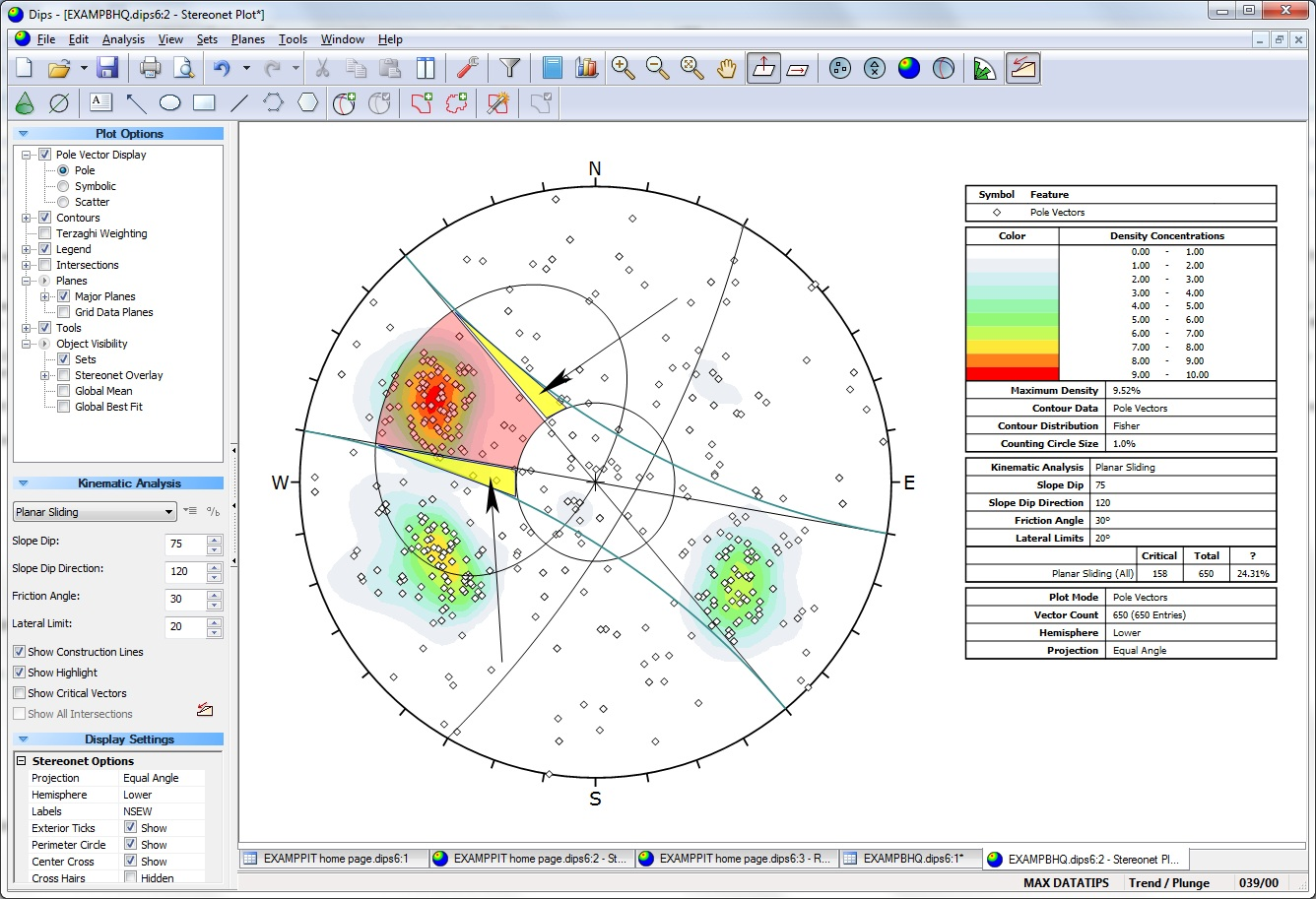
Another consideration is the following. For Planar Sliding, the difference between straight and curved limits becomes more pronounced as the dip angle of a failure plane decreases. (see image below, highlighted yellow regions). However, the probability of oblique planar failure also decreases as planes become flatter. Therefore, we reason that poles which plot in these yellow regions represent a low probability of failure. Conversely, as you approach the stereonet perimeter, the straight and curved lateral limits converge to the same point. Poles plotting near the perimeter (steeply dipping planes) are of the most concern and have the highest probability of oblique failure. For this case, the straight and curved limits are virtually identical (e.g. consider vertical or near vertical slopes).

For Flexural Toppling, the logic is the same. Since the critical poles are near the perimeter, there is virtually no difference between the use of straight or curved limits.

In general, we feel that straight line limits are sufficient for most analyses and are easier to understand and implement.

You can still draw a curved lateral limit by hand using the cone tool. You need to use a pole vector plot for this. For a lateral limit of X degrees, you should draw a cone with radius of 90-X degrees, centered at a trend offset 90 degrees from the dip direction of the slope and a plunge of 0. For example, if you are performing a Kinematic Analysis with 20 degree lateral limit and a slope with dip/dip direction of 75/230 you would place a cone with radius 70 at trend/plunge of 140/0.

You will need to either use the planar sliding failure mode with lateral limits and manually count the number of poles that fall in the space between the linear and curved limits, adding them to the total, or use Planar Sliding failure mode without lateral limits and count the number of poles that fall inside the total critical area but outside the curved limits, and subtract them from the total.

Why does Dips occasionally calculate a dip average that is outside the range of dip directions?

The calculation of mean planes from Set Windows is based on vector averaging of the pole vectors. It is not a simple numerical average, as this does not give you the correct results.

For a wrapped set window, it is possible to obtain a mean dip (for example) which is outside the actual range of the individual readings. This is because the poles on the opposite side of the stereonet are actually assigned an upper hemisphere orientation so that the correct mean vector is obtained. See the note about mean vector calculation for Wrapped Set Windows.

In general, straight numerical averaging of orientation data is not recommended and should be used with caution. For example, with trend values on either side of 0/360, numerical averaging will give wrong answers.

Details of the mean vector calculation in Dips can be found in the Verification Manual.

I need to know how you have discretized the equal area net used for contouring the poles. A standard equal area net would result in biasing the pole count and the contours. Chapter 3 of Rock Slope Engineering has a reference to Denness. Is this the method used in Dips?

First and foremost, it is important to note that all calculations in Dips regarding pole densities, etc, take place ON THE REFERENCE HEMISPHERE, and NOT on the 2-dimensional stereonet. This avoids all of the problems associated with the various methods of determining contours directly on the 2D stereonet, and is in fact much simpler to program and understand.

In Dips, the pole concentration contours are determined as follows:

First, a regular, square grid is superimposed on the 2D stereonet. (In the old DOS version of Dips, the grid spacing could be set to one of two values: 4% or 6% of the projection radius. In the Windows version of Dips, the spacing is fixed at 4%, since a finer grid spacing gives smoother and more accurate contours).

1. This square grid of points is then back-mapped onto the reference hemisphere, resulting in a corresponding grid of points on the surface of the sphere. This is the actual grid used in the contouring calculations.
2. Each pole is assigned an influence on the surface of the sphere, according to the Distribution method used - Fisher or Schmidt.
3. A "floating cone" is then used, such that its circular intersection on the surface of the sphere, encloses an area equivalent to 1% of the area on ONE hemisphere. (1% is the default, and commonly used value, however, the user can set different values if desired, between 0.5% and 5%, using the Count Circle option in the Stereonet Options dialog.
4. This circle (or cone) is then centered on each grid point on the sphere, and the pole vectors falling within the cone are counted (using either the Schmidt or Fisher influence for each pole), and the total at each grid point is divided by the total population, to obtain a concentration value (density) at each grid point on the sphere.
5. Once the grid point densities on the sphere have been calculated, the grid values are assigned to the associated grid points on the 2D stereonet. This square array of values is then contoured using linear interpolation in 2 dimensions, to generate the continuous contours that you see in Dips.

NOTES:

• The "floating cone" used in Dips is analogous, in 3D, to the "floating circle" counting method described in Rock Slope Engineering. However, distortion and data loss are completely eliminated, since the counting is done on the sphere and not on the projection. (2D grid cell methods such as the Denness method, are NOT used in Dips.)
• If you are using Traverses in your Dips file, note that both WEIGHTED (Terzaghi bias correction applied) and UNWEIGHTED densities are calculated at each grid point. This produces the WEIGHTED contour plot in Dips. If you are not using Traverses, then weighted and unweighted plots will appear the same.
• See as well the Density Calculation topic.

What are the confidence and variability limits in Dips and how are they calculated?

The formulae for the confidence and variability limits used in Dips, are as follows:

• Variability limit angle:
  
  cos(alpha) = 1.0 + ln(1-P)/(K)
• Confidence limit angle:
  
  cos(alpha) = 1.0 + ln(1-P)/(RK)

where P is one of 2 probabilities:

• For variability, it is the probability that a vector selected at random makes a solid angle of theta with the calculated mean.
• For confidence, it is the probability that the calculated mean is within theta of the true population mean.

P in the above formulae ranges from 0 to 1 (i.e. 0 % to 100%)

K and R are defined as follows:

K is Fisher's constant = (N - 1) / (N - R)

where N is the total length of pole vectors in a set, and R is the length of the resultant vector (upon vector addition of all poles in the set)

NOTE:

• The numerical value of Fisher's constant K, for each set that you have created, can be found in the Info Viewer listing in Dips.
• The values of N and R are derived from the mean vector calculation for a set. Since we consider a sphere of unit radius, each pole vector is of unit length, and therefore the value of N is numerically equal to the number of poles in the set. The value of R is the length of the resultant vector, upon vector addition of all poles in a set (therefore the value of R is always less than or equal to the value of N). The orientation of vector R, is the mean orientation for the set.

A reference for these calculations, is the following:

Priest, S.D. (1985) Hemispherical projection methods in rock mechanics. London: George Allen & Unwin. 124p.

The formulae are calculated as described in Section 5.4 pages 44 to 50 (Variability: Equations 5.17 and 5.18, Confidence: Equations 5.19 and 5.20)

For more detailed information, you can track down this reference.

See as well the Set Statistics topic.