5 - Qualitative/Quantitative Analysis
1.0 Introduction
The tutorial uses the example file Examppit.dips9. The data has been collected by a geologist working on a single rock face above the first bench in a young open pit mine.
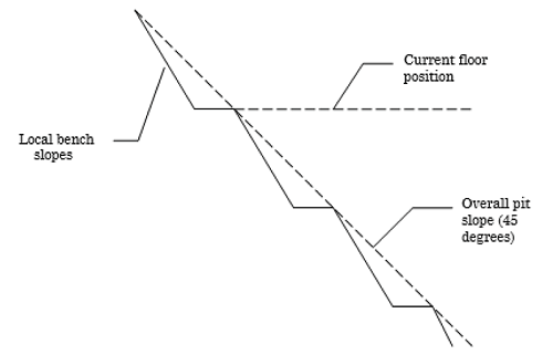
The rock face above the current floor of the existing pit has a dip of 45 degrees and a dip direction of 135 degrees. The current plan is to extend the pit down at an overall angle of 45 degrees. This will require a steepening of the local bench slopes, as indicated in the figure above. The local benches are to be separated by an up-dip distance of 16 m. The bench roadways are 4 m wide.
Topics Covered in this Tutorial:
- Units
- Manual Cluster Analysis
- Symbolic Plot
- Qualitative/Quantitative Chart
Finished Product:
The finished product of this tutorial can be found in the Tutorial 05 Qualitative and Quantitative Analysis.dips9 file, located in the Examples > Tutorials folder in your DIPS installation folder.
2.0 Model
If you have not already done so, run DIPS by double-clicking on the DIPS icon in your installation folder. Or from the Start menu, select Programs > Rocscience > DIPS > DIPS.
If the DIPS application window is not already maximized, maximize it now, so that the full screen is available for viewing the model.
DIPS comes with several example files installed with the program. These example files can be accessed by selecting File > Recent > Examples Folder from the File menu (or File > Open from the Home ribbon). This tutorial will use the Examppit.dips9 file to demonstrate the basic plotting features of DIPS.
- Select File > Recent > Example Folder
 from the menu.
 - Open the Examppit.dips9 file. Since we will be using the Examppit.dips9 file in other tutorials, save this example file with a new file name without overwriting the original file.
- Select File > Save As
 from the menu.
 - Enter the file name Tutorial 05 Qualitative and Quantitative Analysis and Save the file.
3.0 Pole Data Grid
If the Pole Data Grid is not already the active view:
- Select the Pole Data Grid
 view tab.
You should see the Pole Data Grid view shown in the following figure.
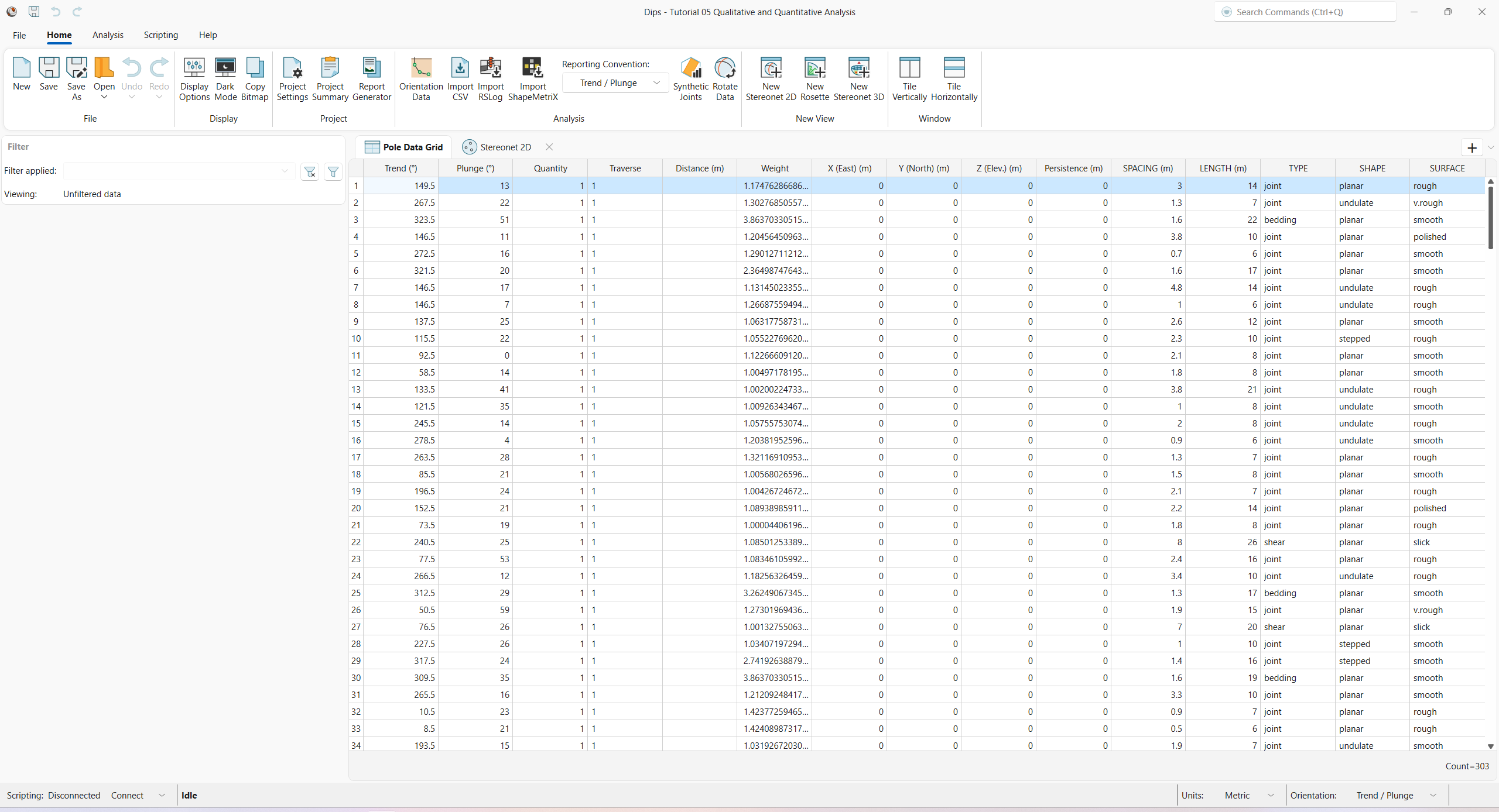
The Pole Data Grid shows all processed orientation data entered in the Orientation Data dialog. Note that there are 303 rows of data (i.e., Count=303) and the following columns:
- Trend and Plunge columns showing the processed orientations in the selected Reporting Orientation.
- Quantity column
- Traverse column
- Distance column
- Weight column
- X (East) column
- Y (North) column
- Z (Elev.) column
- Persistence column
- Five extra columns (i.e., SPACING, LENGTH, TYPE, SHAPE, SURFACE)
3.1 Project Settings
The Project Settings contain options for the Reporting Conventions of Units and Orientation.
- Select Home > Project > Project Settings
 from ribbon. The Project Settings
dialog appears.
from ribbon. The Project Settings
dialog appears. - Units = Metric. All units are converted to the equivalent metric units (e.g., Length as m)
- Orientation = Dip / Dip Direction. All planar orientations are converted to the equivalent orientation format.
3.2 Orientation Data
The Orientation Data dialog is the primary data input for DIPS orientation data. To review the raw, unprocessed input data:
- Select Home > Analysis > Orientation Data
 from the ribbon.
 - The Orientation Data
dialog appears.
- Note that there is one dataset (or traverse).
- Select dataset 1.
- The Name = 1 and acts as its unique identifier and is used for traverse associations in the Traverse column of the Pole Data Grid.
- The Type = Planar Mapping. See the Traverse Types topic for more information.
- In the Traverse tab:
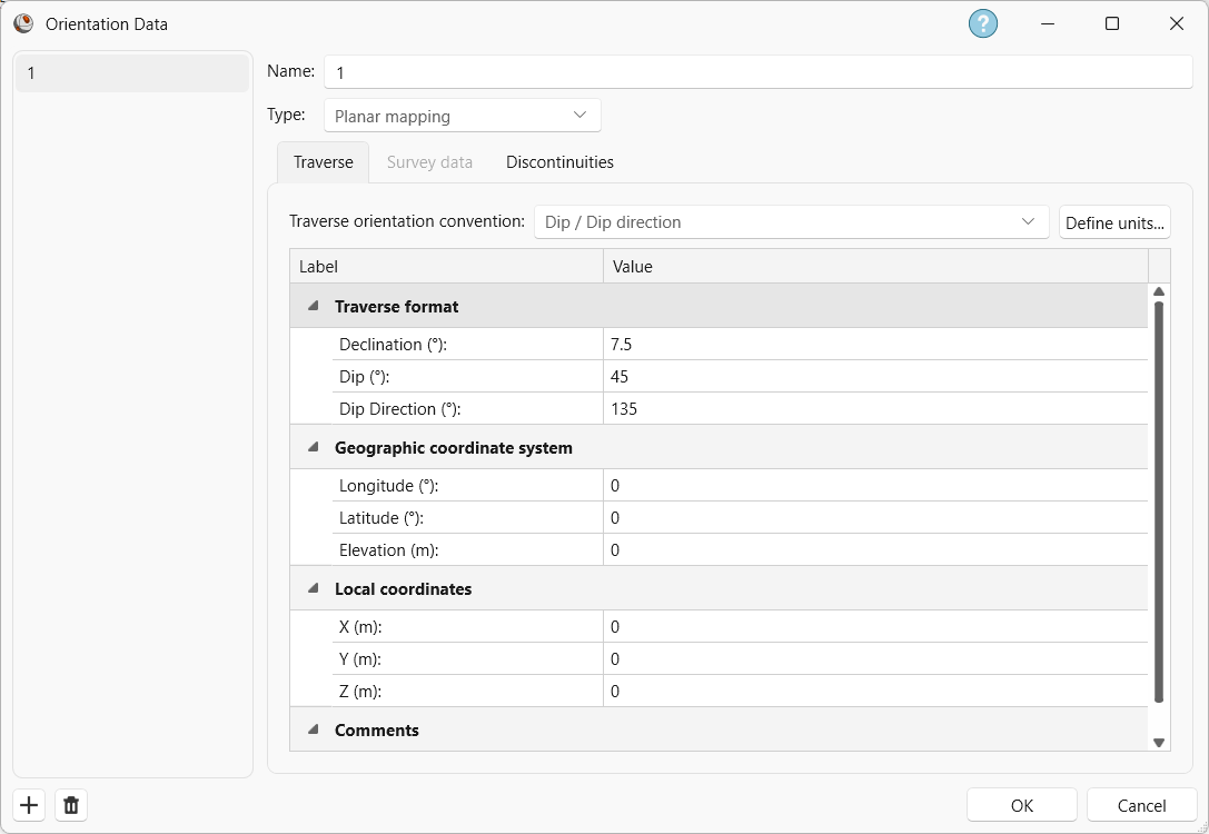
Dataset 1 Traverse tab in the Orientation Data dialog - Traverse Orientation Convention = Dip / Dip Direction.
- Declination = 7.5 degrees, indicating that 7.5 degrees will be added to the Dip Direction of the data, to correct for magnetic declination. See the Declination topic for more information.
- Dip = 45 degrees.
- Dip Direction = 135 degrees. See the Traverse and Traverse Format topics for more information.
- Comment = SECTOR N-45-W-200, face above survey bench.
- In the Discontinuities
tab:
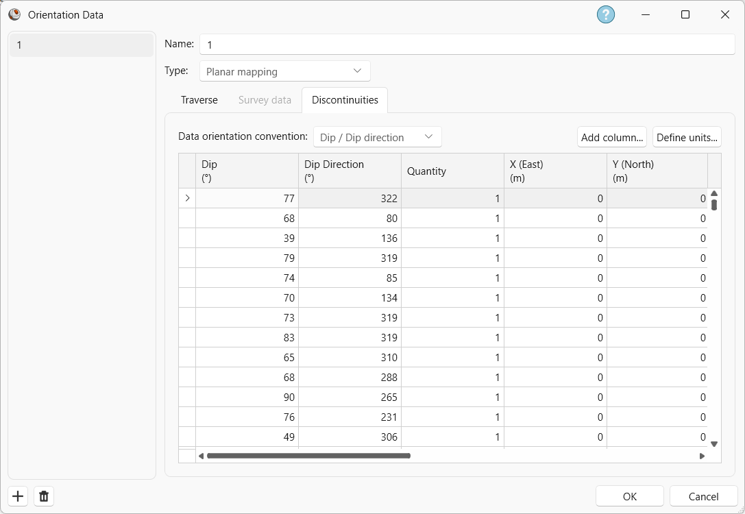
Dataset 1 Discontinuities tab in the Orientation Data dialog - Data Orientation Convention = Dip / Dip Direction. This dictates the orientation format of the first two columns.
- There are 303 rows of discontinuity data.
- Select the Define Units button.
- The Define Units dialog appears, showing all unit-sensitive and user-defined extra columns.
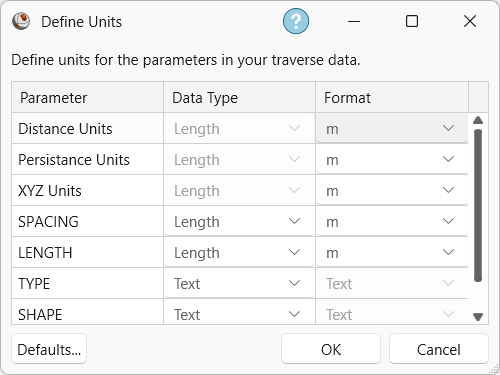
Define Units dialog - Note Data Type and Format of SPACING and LENGTH columns. These extra columns are numeric (i.e., quantitative) and unit-sensitive, representing Length as m.
- Note the Data Type of TYPE, SHAPE, and SURFACE columns. These extra columns are Text (i.e., qualitative) attributes.
- Select Cancel to close the Define Units dialog.
- Select Cancel to close the Orientation Data dialog.
4.0 Stereonet 2D
Now look at the Stereonet 2D view:
- Select the Stereonet 2D
 view tab.
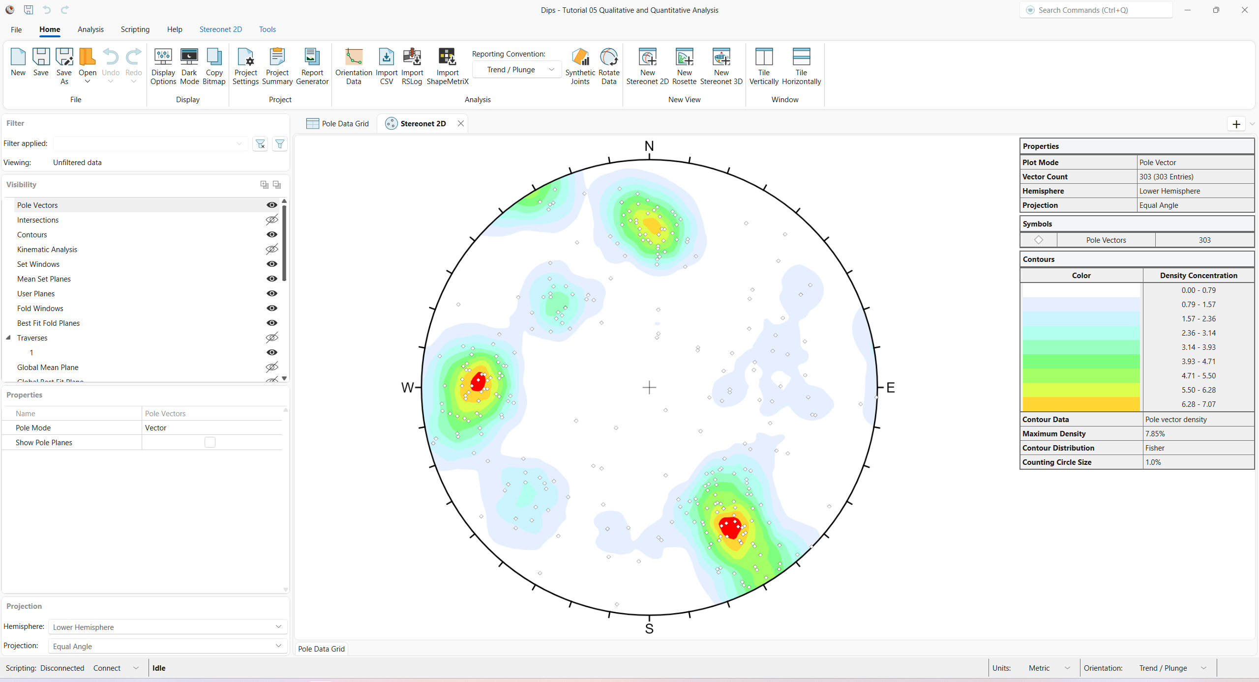
You should see the Stereonet 2D view shown in the following figure.
5.0 Symbolic Pole Plot
Feature attribute analysis can be carried out on a Pole Plot with the Symbolic Plot option. Let’s create a Symbolic Pole Plot based on the discontinuity type (i.e., the data in the TYPE column).
- Select Stereonet 2D > Preset > Symbolic
 from the ribbon. The Symbolic Options dialog appears.
 - Set Data Column = TYPE from the drop down.
- The Data Type = Qualitative. The TYPE column cannot be Quantitative since the Data Format is non-numeric.
- Under the Allocated Items, ensure that bedding, joint, and shear are selected.
- Click OK to generate the Symbolic Plot.
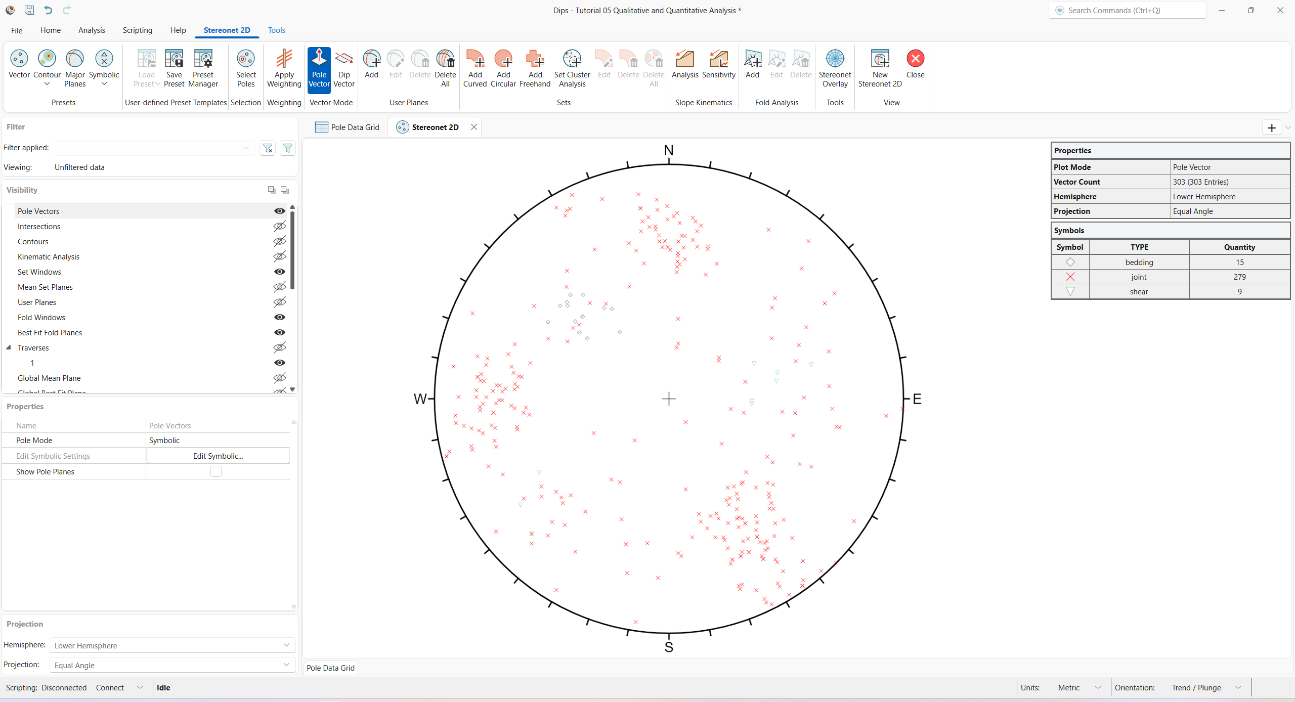
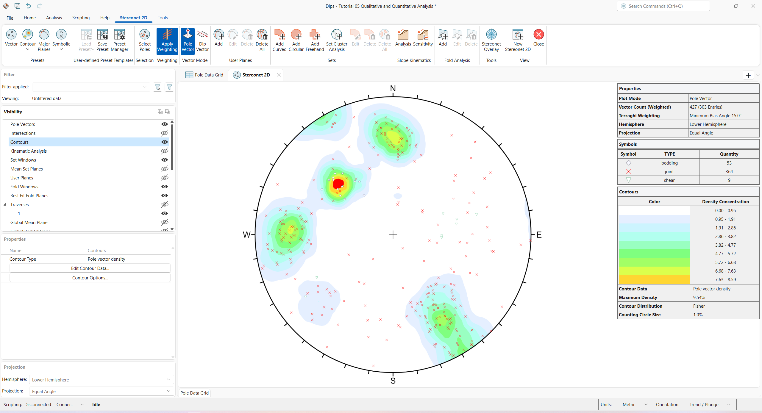
Look closely at the data clustering and the data TYPE. Most of the features are joint as indicated in the Legend.
6.0 Contour Plot
Overlay contours in conjunction with pole symbols.
- Turn on Contours Visibility
 from the Visibility pane.
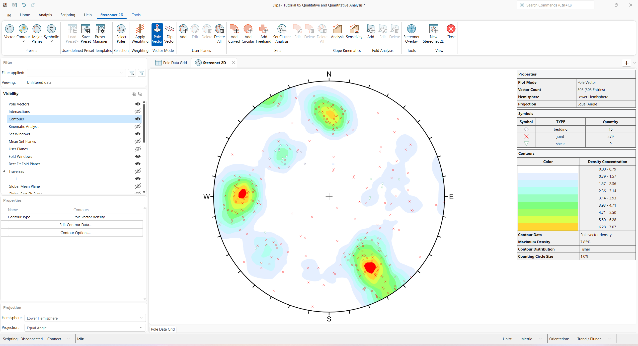
Note the clustering of bedding features and the two clusters of shear features. These may behave very differently from similarly oriented joints or extension fractures and should be considered separately.
Although the shear features are not numerous enough to be represented in the contours (the number of mapped shears is small), they may have a dominating influence on stability due to low friction angles and inherent persistence. It is always important to look beyond mere orientations and densities when analyzing structural data.
A useful rule of thumb is that any cluster with a maximum concentration of:
- Greater than 6% is very significant.
- 4-6% represents a marginally significant cluster.
- Less than 4% should be regarded with suspicion unless the overall quantity of data is very high (several hundreds of poles).
Rock mechanics texts give more rigorous rules for statistical analysis of data.
Now apply the Terzaghi Weighting to the data to account for bias correction due to data collection on the (Planar) Traverse.
- Select Stereonet 2D > Weighting > Apply Weighting
 from the ribbon.
Observe the change in adjusted concentrations for each cluster, particularly the cluster dominated by the bedding attribute.
- Deselect Stereonet 2D > Weighting > Apply Weighting from the ribbon.
See the Terzaghi Weighting topic for more information.
7.0 Sets from Manual Cluster Analysis
Use the Manual Cluster Analysis option to quickly delineate contours and create four Sets from the four major data concentrations on the stereonet.
- Select Stereonet 2D > Sets > Set Cluster Analysis
 from the ribbon. The Manual Cluster Analysis
dialog appears.
from the ribbon. The Manual Cluster Analysis
dialog appears. - Enter Limit Cluster Size to Cone with Maximum Angle = 25 degrees.
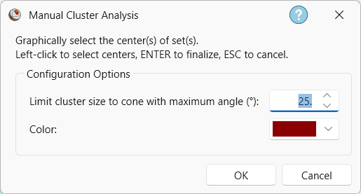
Manual Cluster Analysis dialog - Click OK to start graphically selecting centers of sets.
- Left-click the mouse button to pick the approximate center of the four main data clusters on the stereonet.
- Hit ENTER (or right-click > Done) to finalize the Sets.
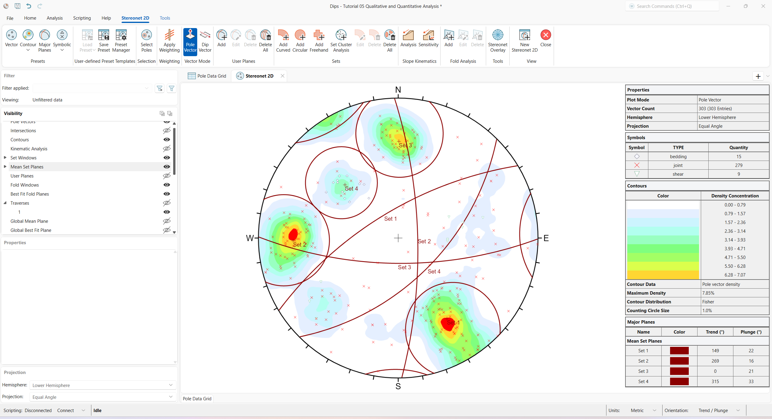
Turn on the display of Mean Set Planes and the Major Planes Legend:
- Turn on the Mean Set Planes
group Visibility from the Visibility tree.
You should see the Circular Set Windows shown below.
8.0 Qualitative Chart
Aside from graphical representations of Pole or Vector Symbolic Plots in a stereonet, DIPS also provides charting capabilities for Qualitative/Quantitative Analysis.
- Select Analysis > Qualitative/Quantitative > Chart
 from the ribbon. The Qualitative/Quantitative Analysis dialog appears.
 - Set Data Column = SURFACE.
- The Data Type = Qualitative. The SURFACE column cannot be Quantitative since the Data Format is non-numeric.
- Under the Allocated Items, ensure that polished, rough, slick, and v.rough are selected.
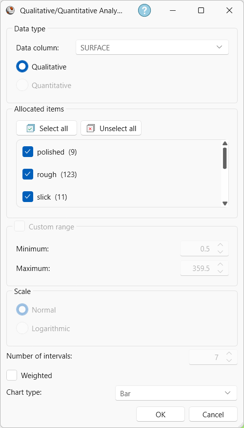
Qualitative/Quantitative Analysis dialog - Set Chart Type = Bar from the drop down.
- Click OK to generate the Qualitative chart.

There is no single, dominating SURFACE attribute.
TIP: More insight can be gathered by plotting the SURFACE attribute for each Set. This can be accomplished with Data Filters, which will be left as an optional exercise.
This concludes the tutorial. You are now ready for the next tutorial, Tutorial 06 – Kinematic Analysis.