9 - Data Filters
1.0 Introduction
This tutorial demonstrates the use of the Data Filters when working with subsets of Pole Data Grid entries. While working in a DIPS file, Pole Data can be either queried to generate a new DIPS file of the subset of data or dynamically filtered by view in the current DIPS file.
Topics Covered in this Tutorial:
- Filter Options
- Applying and Toggling Filters
- Creating a New DIPS File with Data Query
Finished Product:
The finished product of this tutorial can be found in the Tutorial 09 Data Filters.dips9 file, located in the Examples > Tutorials folder in your DIPS installation folder.
2.0 Model
If you have not already done so, run DIPS by double-clicking on the DIPS icon in your installation folder. Or from the Start menu, select Programs > Rocscience > DIPS > DIPS.
If the DIPS application window is not already maximized, maximize it now, so that the full screen is available for viewing the model.
DIPS comes with several example files installed with the program. These example files can be accessed by selecting File > Recent > Examples Folder from the File menu (or File > Open from the Home ribbon). This tutorial will use the Data Filters.dips9 file to demonstrate the basic plotting features of DIPS.
- Select File > Recent > Example Folder
 from the menu.
 - Open the Dynamic Filter.dips9 file. Since we will be using the Dynamic Filter.dips9 file in other tutorials, save this example file with a new file name without overwriting the original file.
- Select File > Save As
 from the menu.
 - Enter the file name Tutorial 09 Data Filters and Save the file.
3.0 Pole Data Grid
If the Pole Data Grid is not already the active view:
- Select the Pole Data Grid
 view tab.
You should see the Pole Data Grid view shown in the following figure.
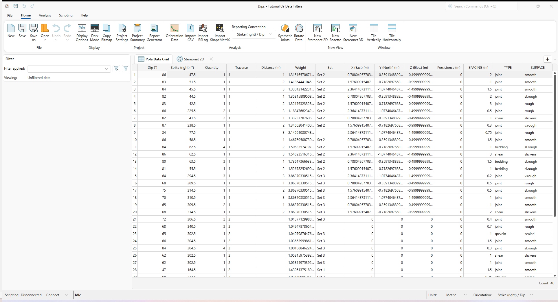
The Pole Data Grid shows all processed orientation data entered in the Orientation Data dialog. Note that there are 40 rows of data (i.e., Count=40) and the following columns:
- Trend and Plunge columns showing the processed orientations in the selected Reporting Orientation.
- Quantity column
- Traverse column
- Distance column
- Weight column
- Set column
- X (East) column
- Y (North) column
- Z (Elev.) column
- Persistence column
- Three extra columns (SPACING, TYPE, SURFACE)
Any of these columns can be used to query a subset of the data using the Data Filter feature of DIPS.
4.0 Data Filters
The Data Filters feature in DIPS allows users to easily and dynamically query the data displayed and used for analysis in all views (i.e., Pole Data Grid, Stereonet 2D, Stereonet 3D, Rosette, Chart).
To manage Data Filters:
- Select the Filter Options
 button from the Filter pane.
 - The Filter Options
dialog appears. Seven Data Filters are defined.
- All Joints
- Joints with Rough Surface
- Joints with Rough Surface and Spacing Less Than 1
- All Faults and Shears
- Spacing between 0.5 and 1.5
- Joints in Traverse 1 and 2
- Set 1
- Select each Data Filter to review the conditional statements that define the query. Data Filters can be simple single conditional statements (e.g., Set 1) or can be complex and contain several conditional statements tied together by “AND” and “OR” logical operators (e.g., Joints in Traverse 1 and 2).
- Click the Add New Filter
 button.
- Enter Name = Set 2. The Name must be unique across all Data Filters in the DIPS project.
- Click the + button.
- Select Field Name = Set in the drop down. A list of all available columns in the Pole Data Grid is available, including all processed Orientation conventions (i.e., Trend, Plunge, Dip, Dip Direction, Strike (right), Strike (left)).
- Select Criteria Operator = Equals in the drop down.
- Enter or select Operand Value = Set 2 in the drop down. A list of all available column values in the Pole Data Grid is available for the selected Field Name (i.e., column name).
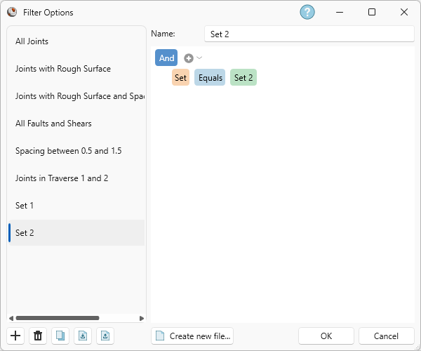
Filter Options dialog - Enter Name = Set 2.
- Click OK.
TIP: Any Data Filter can be selected and used to create a new DIPS file with only entries matching the filter criteria by clicking the Create New File button in the Filter Options dialog. This will be left as an optional exercise.
4.1 Filter Applied
By default, no filter is applied, which displays as Viewing: Unfiltered data in the Filter pane.
To apply a Data Filter:
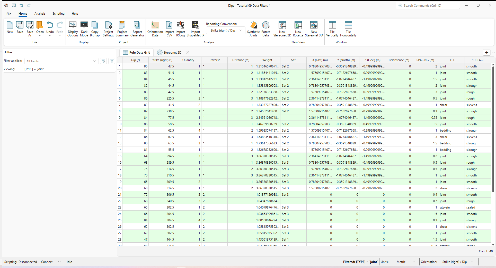
- Set Filter Applied = All Joints from the drop down in the Filter pane.
Note the following when a Data Filter is Applied:
- The conditional statement Viewing: [TYPE] = ‘joint’ is shown under the Filter Applied drop down, and Filtered: [TYPE] = ‘joint’ is shown in the Status Bar.
- Rows of the Pole Data Grid matching the Data Filter are highlighted in LIGHT GREEN.
Toggle through the various filters to see how they apply.
Clear the filter:
- Select the Clear Filter
 button from the Filter pane.
5.0 Stereonet 2D
Now look at the Stereonet 2D view:
- Select the Stereonet 2D
 view tab.
You should see the Stereonet 2D view shown in the following figure.
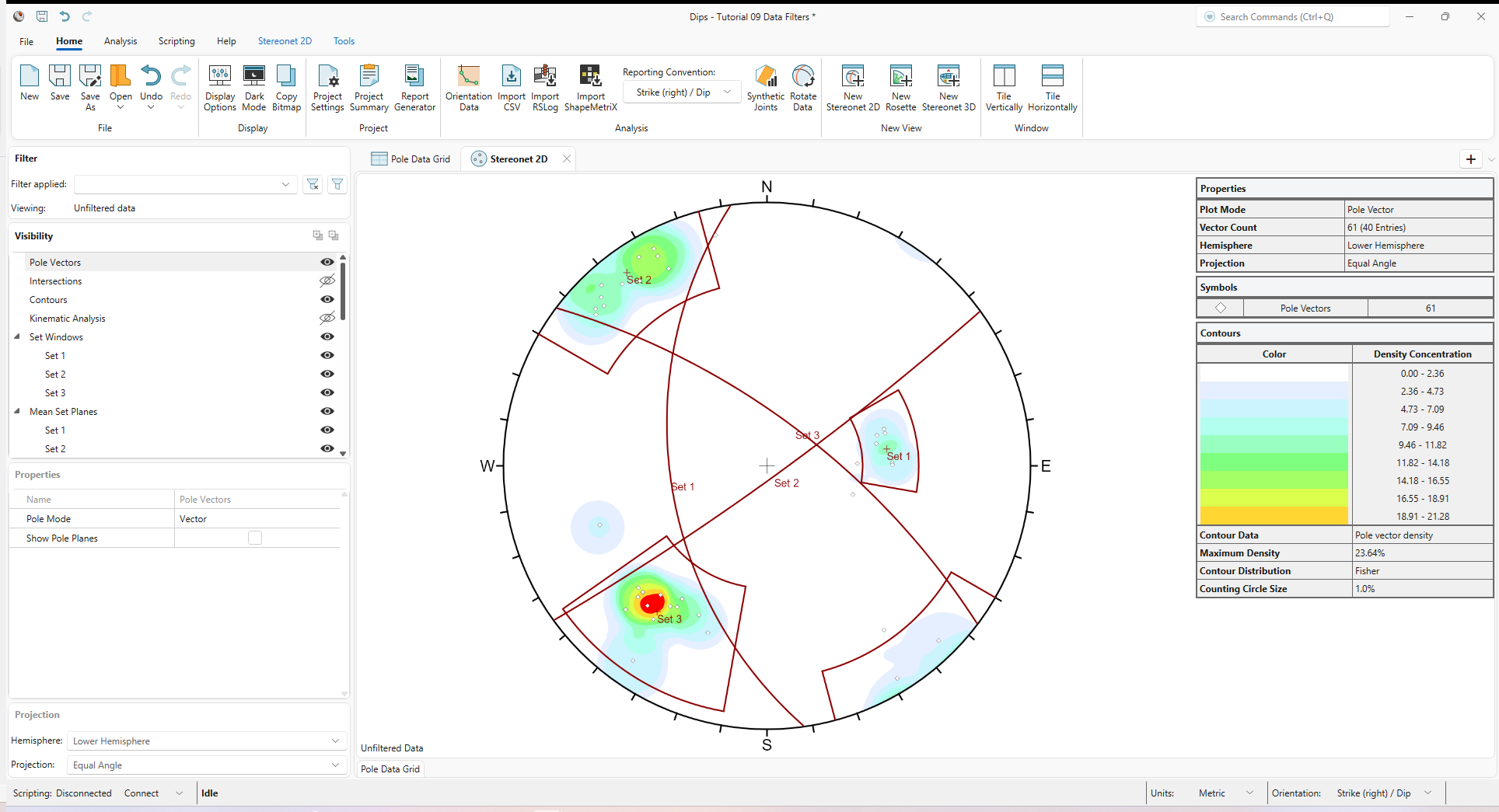
Just like the Pole Data Grid view, a Data Filter can be applied to any view in DIPS, including the Stereonet 2D view.
To apply a Data Filter:
- Set Filter Applied = All Joints from the drop down in the Filter pane.
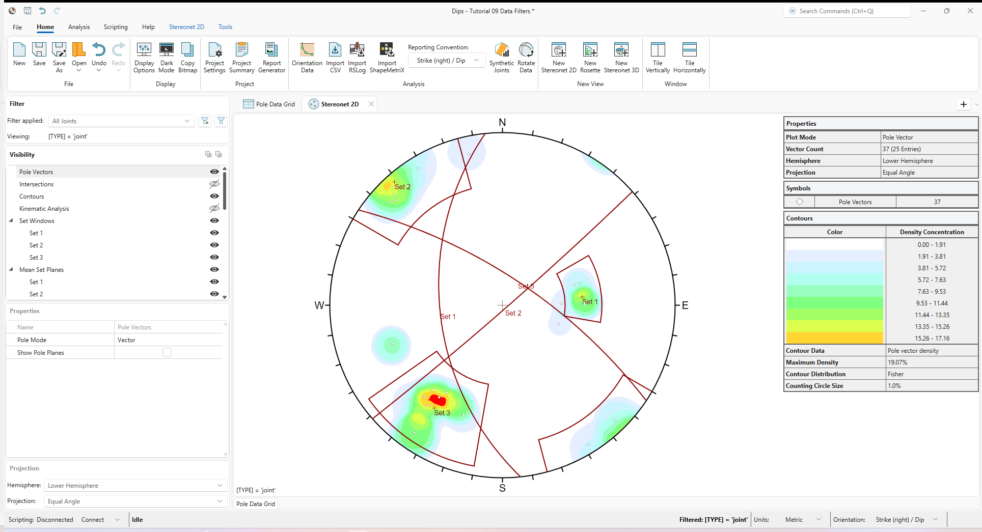
Stereonet 2D view showing “All Joints” filter applied Only poles associated with [TYPE] = ‘joint’ are shown, and the Contours, Mean Set Planes, and Legend are updated to show the results for this Data Filter. - Set Filter Applied = Set 1
from the drop down in the Filter pane.
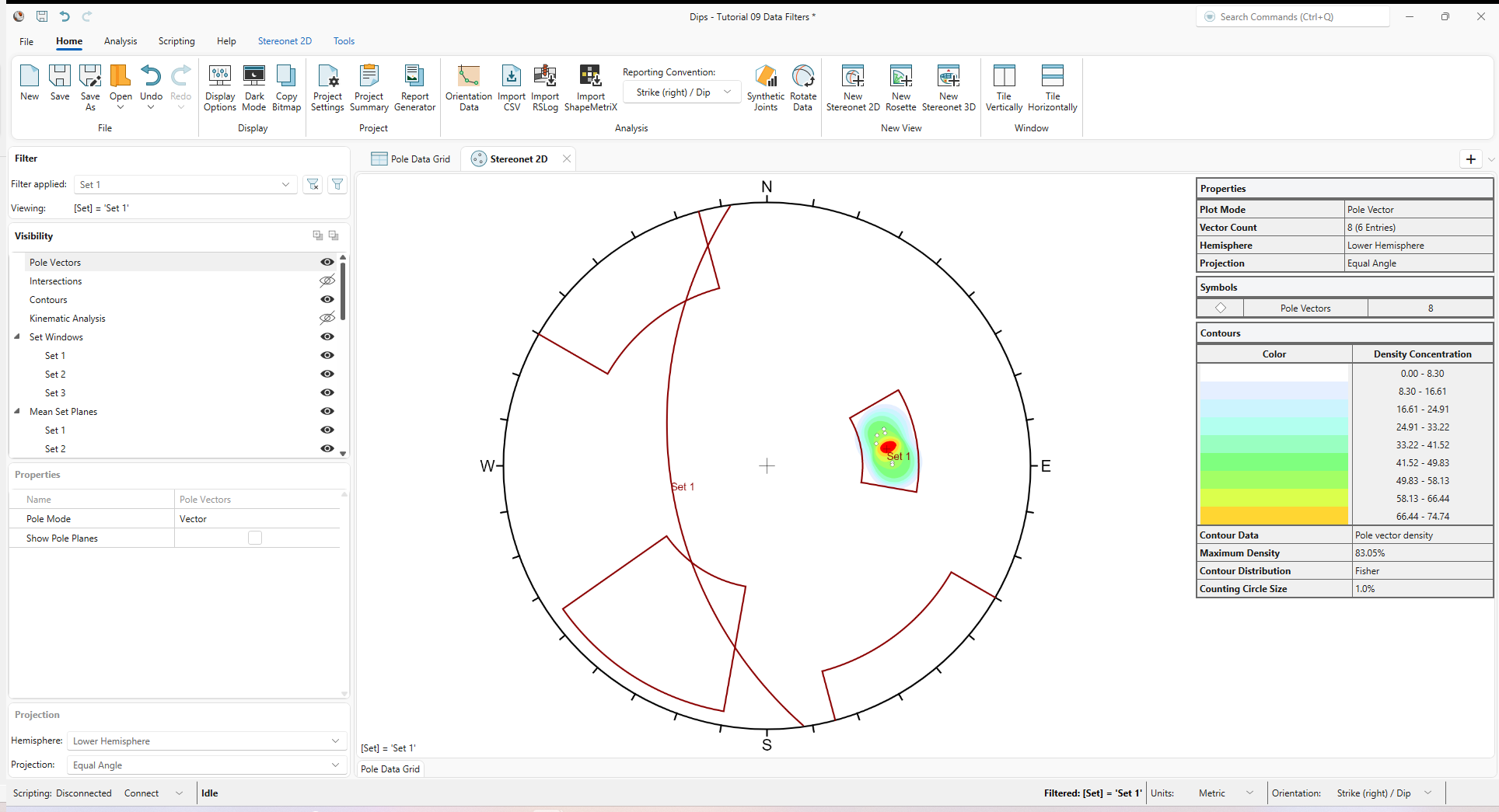
Stereonet 2D view showing “Set 1” filter applied Set 2 and Set 3 contain no poles when [Set] = ‘Set 1’ filter is applied. Set statistics have no meaning for Sets containing no poles; therefore, the Mean Set Planes are not calculated or shown for Set 2 and Set 3.
Data Filters are view-specific. Changing filters in the Filter Applied drop down list in the Filter pane affects the active view only.
WARNING: Be careful when adding Sets in a filtered view, as the Pole Vectors and Contours reflect only what is in the filtered subset of poles.
6.0 Chart View
Like the Pole Data Grid view and the Stereonet 2D view, any active Chart view can also be toggled independently of other open views. This will be left as an additional exercise.
Keep in mind that viewing filtered results for various analysis types can be done by toggling the Filter Applied drop down in the Filter pane.
- Kinematic Analysis
- Kinematic Sensitivity
- Quantitative or Qualitative Charts
- Joint Spacing
- RQD Analysis
- Frequency Analysis
- Histogram
- Cumulative
- Scatter
7.0 Report Generator
When Data Filters are defined in the DIPS project, the Report Generator will also include the filtered results (in addition to unfiltered results) for:
- Global Best Fit
- Global Mean
- Sets
- Folds
- Intersections
This concludes the tutorial. You are now ready for the next tutorial, Tutorial 10 – Scripting.