6 - Kinematic Analysis
1.0 Introduction
Based on kinematic considerations and frictional properties of joint planes, it is possible to perform stability analyses such as planar sliding, wedge sliding, and toppling on a stereonet. This tutorial demonstrates how to perform stability analyses under Planar Sliding, Flexural Toppling, Wedge Sliding, and Direct Toppling failure modes using the Kinematic Analysis option in DIPS.
This tutorial uses data from Examppit.dips8 and is a continuation of Tutorial 5 – Qualitative and Quantitative Analysis.
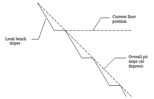
The rock face above the current floor of the existing pit has a dip of 45 degrees and a dip direction of 135 degrees. The current plan is to extend the pit down at an overall angle of 45 degrees. This will require a steepening of the local bench slopes, as indicated in the figure above. The local benches are to be separated by an up-dip distance of 16 m. The bench roadways are 4 m wide.
Topics Covered in this Tutorial:
- Kinematic Analysis
- Kinematic Sensitivity
- Intersections
Finished Product:
The finished product of this tutorial can be found in the Tutorial 06 Kinematic Analysis.dips9 file, located in the Examples > Tutorials folder in your DIPS installation folder.
2.0 Model
If you have not already done so, run DIPS by double-clicking on the DIPS icon in your installation folder. Or from the Start menu, select Programs > Rocscience > DIPS > DIPS.
If the DIPS application window is not already maximized, maximize it now, so that the full screen is available for viewing the model.
DIPS comes with several example files installed with the program. These example files can be accessed by selecting File > Recent > Tutorials Folder from the File menu (or File > Open from the Home ribbon). This tutorial will use the Tutorial 06 Kinematic Analysis_starting file.dips9 file to demonstrate the basic plotting features of DIPS.
- Select File > Recent > Tutorials Folder
 from the menu.
 - Open the Tutorial 06 Kinematic Analysis_starting file.dips9 file. Select File > Save As
 from the menu.
 - Enter the file name Tutorial 06 Kinematic Analysis (Planar Sliding) and Save the file.
3.0 Pole Data Grid
If the Pole Data Grid is not already the active view:
- Select the Pole Data Grid
 view tab.
You should see the Pole Data Grid view shown in the following figure.
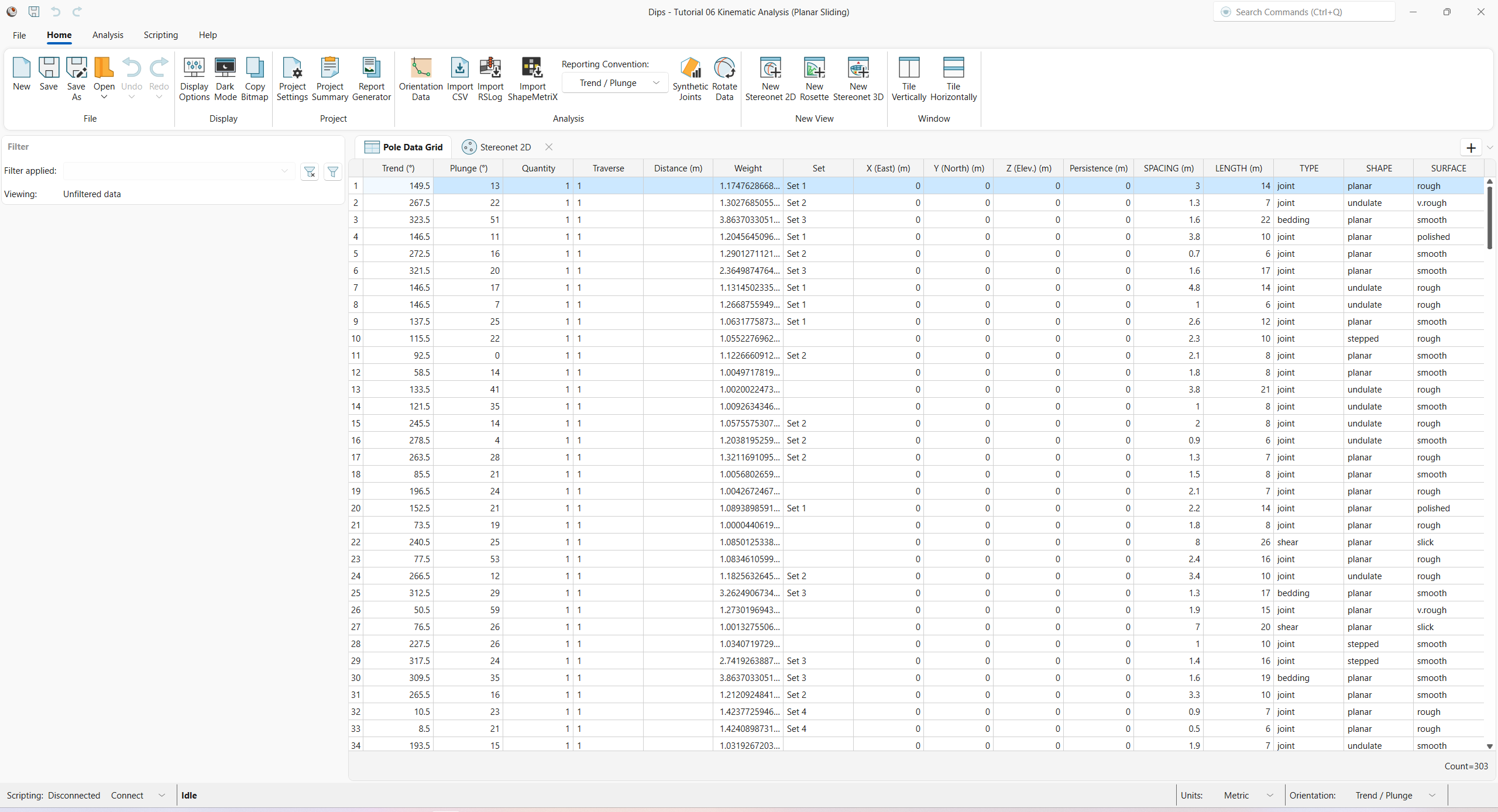
The Pole Data Grid shows all processed orientation data entered in the Orientation Data dialog. Note that there are 303 rows of data (i.e., Count=303).
4.0 Stereonet 2D
Now look at the Stereonet 2D view:
- Select the Stereonet 2D
 view tab.
You should see the Stereonet 2D view shown in the following figure.
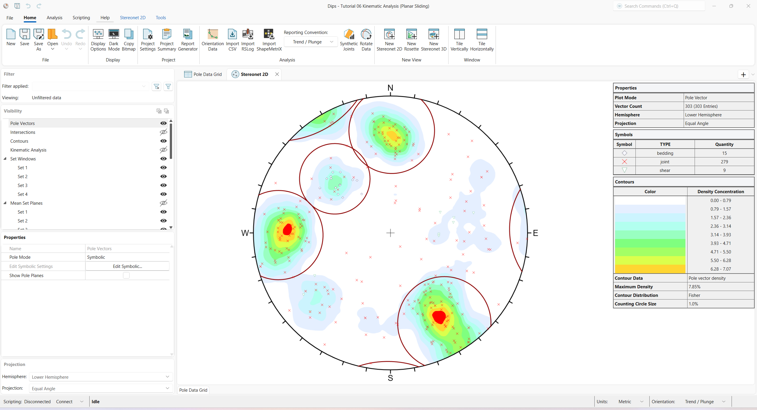
Note that there are four Sets.
5.0 Kinematic Analysis
Kinematic Analysis in DIPS serves to identify critical planes and/or critical plane intersections for the failure mode(s) of interest.
See the Kinematic Analysis topic for more information.
5.1 Planar Sliding
To analyze the Planar Sliding failure mode:
- Select Stereonet 2D > Slope Kinematics > Analysis
 from the ribbon. The Kinematic Analysis
dialog appears.
from the ribbon. The Kinematic Analysis
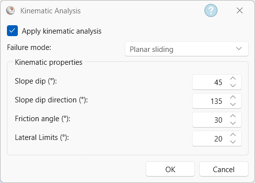
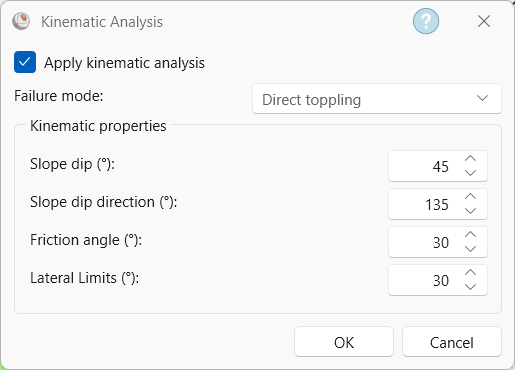
dialog appears. - Select the Apply Kinematic Analysis checkbox. The Kinematic Analysis overlay appears in the Stereonet 2D view.
- Set Failure Mode = Planar Sliding (No Limits) from the drop down.
- Enter Slope Dip = 45 degrees.
- Enter Slope Dip Direction = 135 degrees.
- Enter Friction Angle = 30 degrees.
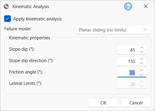
Kinematic Analysis dialog - Click OK to close the dialog and compute Kinematic Analysis.
You should see the Kinematic Analysis overlay for Planar Sliding (No Limits) as shown below.
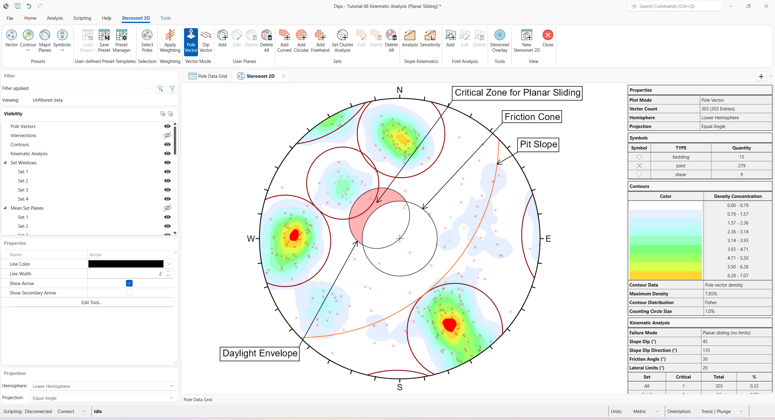
- The text labels in the figure were manually added using the Tools > Annotation > Text option in the ribbon.
- The arrows in the figure were manually added using the Tools > Annotation > Arrow option in the ribbon.
The key elements of Planar Sliding using pole vectors are:
- Slope Plane and Daylight Envelope
- Pole Friction Cone (angle measured from the center of the stereonet)
- Lateral Limits (optional)
These are discussed below.
5.1.1 Slope Plane
The great circle of the Slope Plane is displayed and labelled “Pit Slope” on the above figure with orientation Dip / Dip Direction = 45 / 135.
5.1.2 Daylight Envelope
The Daylight Envelope corresponding to the slope plane is required for a Planar Sliding Kinematic Analysis, as shown in the above figure. A Daylight Envelope allows us to test for kinematics (i.e., a rock slab must have somewhere to slide into – free space). Any pole falling within this envelope is kinematically free to slide if frictionally unstable.
5.1.3 Friction Cone
A pole Friction Cone of 30 degrees is displayed. Any pole falling outside of this cone represents a plane which could slide if kinematically possible.
5.1.4 Critical Zone For Planar Sliding
The crescent-shaped zone formed by the Daylight Envelope and the pole Friction Cone encloses the region of Planar Sliding. Any poles in this region represent planes which can and will slide (i.e., the critical zone for planar failure is defined by poles), which are:
- OUTSIDE of the pole Friction Cone, and
- INSIDE the Daylight Envelope
This region is automatically highlighted for Planar Sliding analysis as shown in the above figure. The highlight colour and other display options can be customized in the Display Options dialog.
5.1.5 Lateral Limits
In practice, it has been observed that Planar Sliding (and toppling) tends to occur when the Dip Direction of planes is within a certain angular range of the Slope Dip Direction. Typically, a range of plus/minus 20 or 30 degrees is considered, and poles outside of this range represent a low risk.
To add lateral limits to the Kinematic Analysis:
- Select Stereonet 2D > Slope Kinematics > Analysis from the ribbon.
- The Kinematic Analysis dialog appears.
- Select Apply Kinematic Analysis checkbox. The Kinematic Analysis overlay appears in the Stereonet 2D view.
- Set Failure Mode = Planar Sliding from the dropdown.
- Enter Lateral Limit = 30 degrees.
Kinematic Analysis dialog - Click OK to close the dialog and compute Kinematic Analysis.
TIP: Alternatively, select Kinematic Analysis from the Visibility tree, and set the Failure Mode and Lateral Limits directly in the Properties pane.
You should see the following.
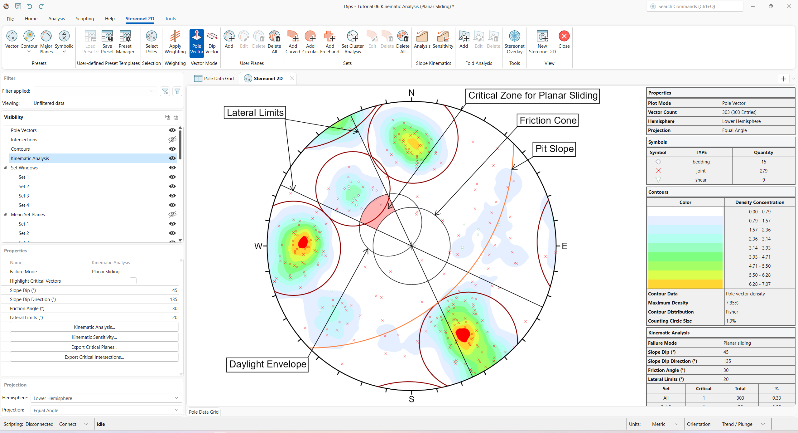
5.1.6 Kinematic Analysis Legend (Results)
A summary of the Planar Sliding Kinematic Analysis results is displayed in the Legend.
In this case, only a single pole is contained within the critical Planar Sliding zone. The Legend provides results as a percentage of all poles in the file (1/303), and as a percentage of poles for individual sets (1/26 for Set 3).
In either case, you can see that the feasibility of Planar Sliding is very low.
5.2 Flexural Toppling
Let’s examine the Flexural Toppling failure mode.
- Select Stereonet 2D > Slope Kinematics > Analysis from the ribbon. The Kinematic Analysis
dialog appears.
- Set Failure Mode = Flexural Toppling from the drop down.
- Enter Lateral Limits = 30 degrees.

Kinematic Analysis dialog - Click OK to close the dialog and compute Kinematic Analysis.
You should see the Kinematic Analysis overlay for Flexural Toppling as shown below.
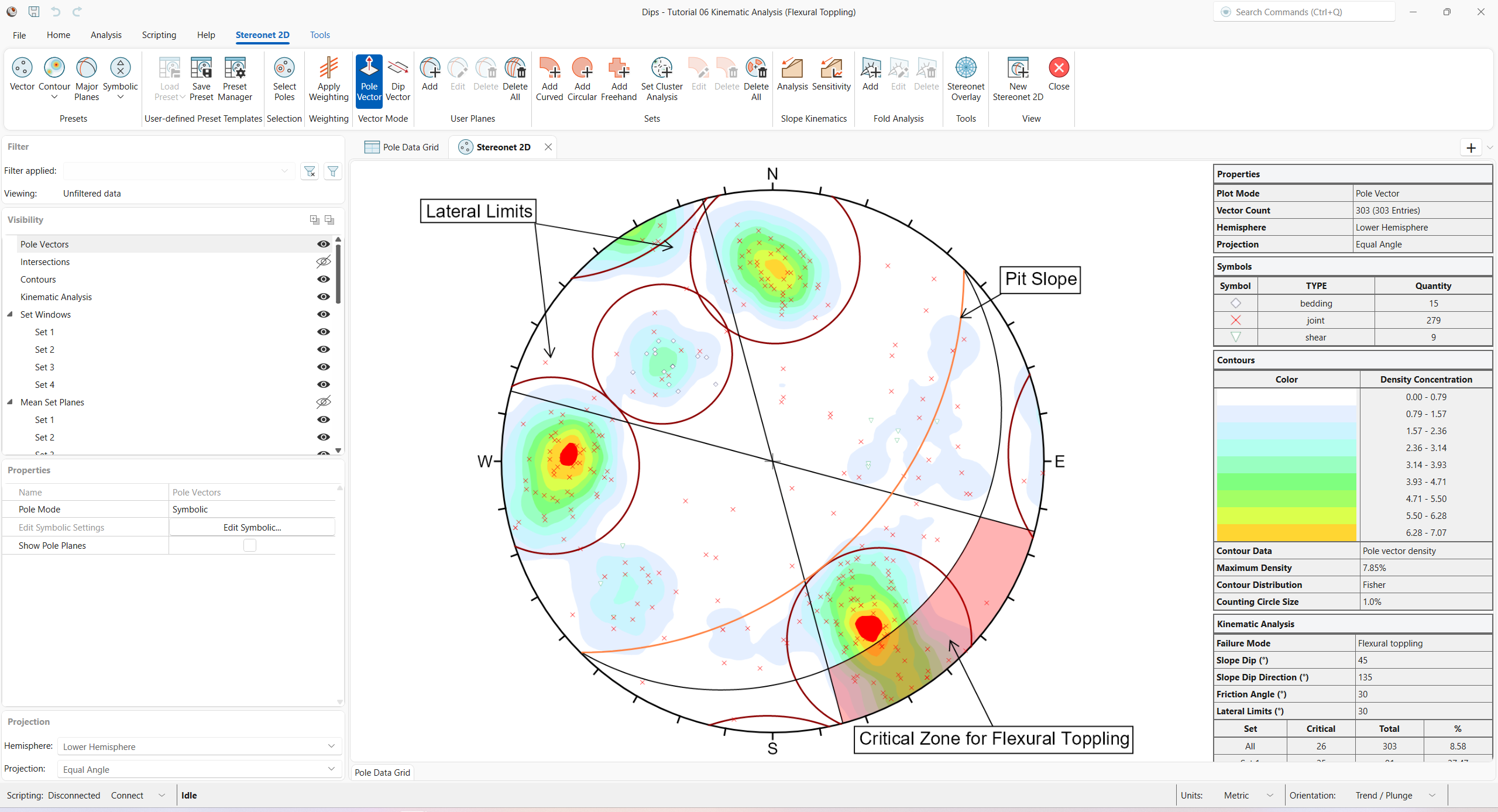
The key elements of Flexural Toppling Kinematic Analysis using pole vectors are:
- Slope Plane
- Slip Limit Plane (based on Slope Dip and Friction Angle)
- Lateral Limits
These are discussed below. Any poles that plot within the critical zone for Flexural Toppling represent a toppling risk. This analysis is based on the Flexural Toppling analysis described by Goodman [1].
5.2.1 Slope Plane
The great circle of the Slope Plane is displayed and labelled Pit Slope with orientation Dip / Dip Direction = 45 / 135.
5.2.2 Slip Limit
Planes cannot topple if they cannot slide with respect to one another. Goodman [1] states that for slip to occur, the bedding normal must be inclined less steeply than a line inclined at an angle equivalent to the Friction Angle above the slope.
This results in a Slip Limit Plane, which defines the critical zone for Flexural Toppling. The Dip angle of the Slip Limit Plane is derived from the following:
Slip Limit Dip = Pit Slope Dip – Friction Angle = 45 – 30 = 15 degrees
The Slip Limit Dip Direction is equal to that of the Slope Dip Direction (135 degrees).
5.2.3 Lateral Limits
The Lateral Limits for Flexural Toppling have the same purpose as described for Planar Sliding. They define the lateral extents of the critical zone with respect to the Slope Dip Direction. For this example, we have increased the limits from 20 degrees (used in the Planar Sliding example) to 30 degrees as suggested by Goodman.
5.2.4 Critical Zone For Flexural Toppling
The Critical Zone for Flexural Toppling is the highlighted region between the Slip Limit Plane, Lateral Limits, and the stereonet perimeter. Any poles in this region represent a risk of Flexural Toppling. Remember that a near horizontal pole represents a near vertical plane.
5.2.5 Kinematic Analysis Legend (Results)
A summary of the Flexural Toppling results is displayed in the Legend.
In this case, there is a significant risk of Flexural Toppling. The Legend provides results as a percentage of all poles in the Pole Data Grid (26/303), and as a percentage of poles for individual sets (25/91 for Set 1). For Set 1, the Flexural percent critical is approximately 27%.
5.3 Wedge Sliding
From the Planar Sliding Kinematic Analysis, it has been shown that a sliding failure along any single joint plane is unlikely. However, multiple joints can form wedges, which can slide along the line of intersection between two planes.
To analyze the Wedge Sliding failure mode:
- Select Stereonet 2D > Slope Kinematics > Analysis from the ribbon. The Kinematic Analysis
dialog appears.
- Set Failure Mode = Wedge Sliding from the drop down.
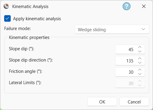
Kinematic Analysis dialog - Click OK to close the dialog and compute Kinematic Analysis.
Since Wedge Sliding pertains to intersection vectors:
- Turn off the Pole Vectors
Visibility
 in the Visibility tree.
 - Select Contours from the Visibility tree.
- Set Contour Type = Intersection Vector Density from the drop down in the Properties pane.
- Turn off the Set Windows group Visibility in the Visibility tree.
- Select Kinematic Analysis from the Visibility tree.
- Select the Highlight Critical Vectors checkbox in the Properties pane.
You should see the Kinematic Analysis overlay for Wedge Sliding as shown below.
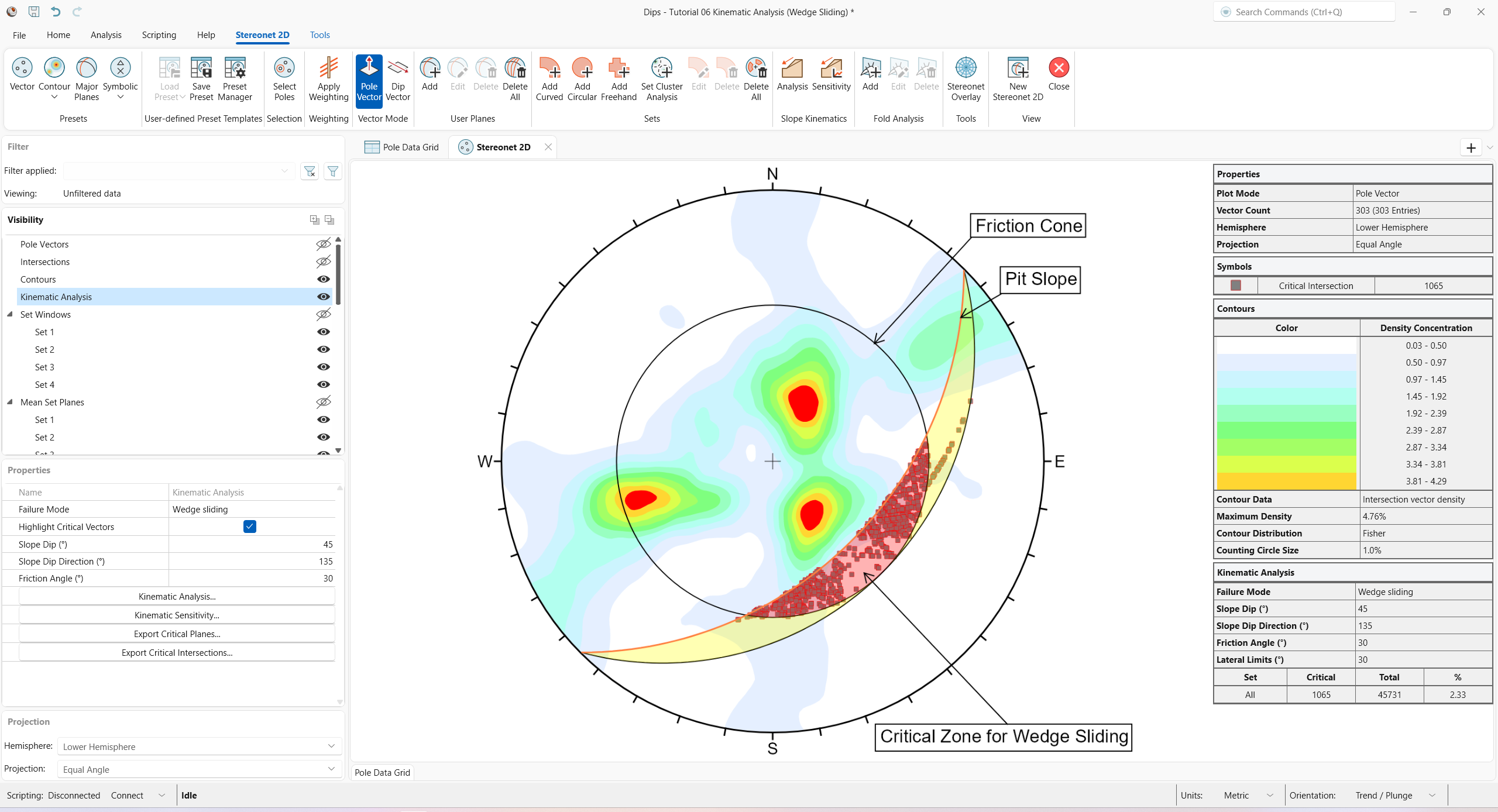
The key elements of Wedge Sliding analysis are:
- Slope Plane
- Plane Friction Cone (angle measured from perimeter of stereonet)
- Intersection plotting
5.3.1 Intersections
The points that you see plotted for the Wedge Sliding analysis are intersection points. Each point represents the intersection of two joint planes. By default, all planes in the Pole Data Grid are considered (i.e., each plane is intersected with every other plane, to determine the intersection points). The intersection points represent the actual Trend/Plunge of the line of intersection of two joint planes. By default, only the critical intersections are displayed.
There are several options available for the display of intersections:
- Pole plane intersections (i.e., intersections between Pole Data Grid planes)
- Major plane intersections (i.e., intersections between Mean Set Planes and/or User Planes).
- Intersection density contours (based on the intersection of all Pole Data Grid planes as shown above)
- Major plane intersections can be plotted (i.e., Mean Set Planes and/or User Planes).
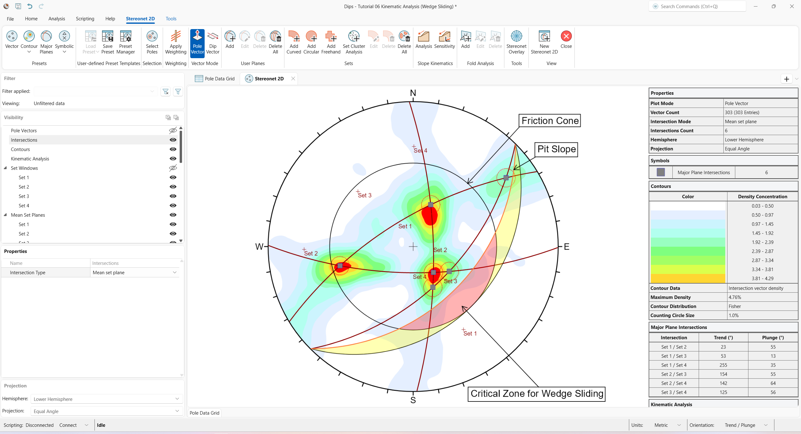
Turn on Pole Intersections visibility:
- Turn on the Intersections
Visibility in the Visibility tree.
Numerous intersections are generated. For a large number of poles, it is generally not practical to visualize all Pole Intersections.
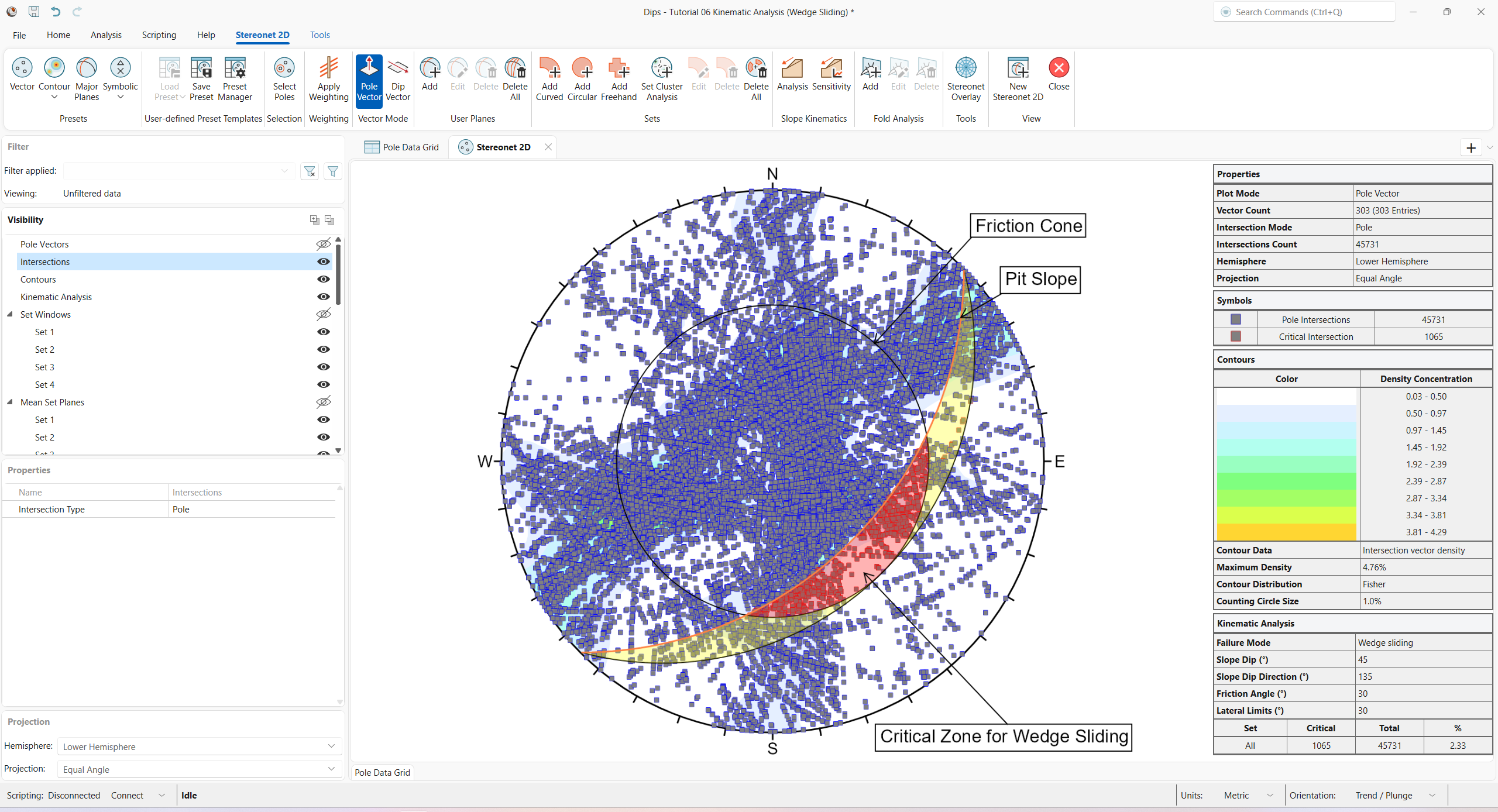
Let’s demonstrate one more possibility for assessing the risk of Wedge Sliding. We will view the intersections of the Mean Set Planes (from the four Sets).
- Turn on the Mean Set Planes
group Visibility in the Visibility tree.
- Select Intersections from the Visibility tree.
- Set Intersection Type = Mean Set Plane from the drop down in the Properties pane.
Notice that the four Mean Set Planes intersect each other to form 6 intersection points. Notice that these intersections correspond with the maximum concentrations of the intersection contours, as we would expect.
Since none of the Mean Set Plane intersections are within the Critical Wedge Sliding Zone, we can conclude that Wedge Sliding is not probable. Note that the Legend indicates 0/6 critical Mean Set Plane Intersections.
Switch back to the display of all intersections:
- Turn off the Mean Set Planes
group Visibility in the Visibility tree.
- Turn off the Intersections
Visibility in the Visibility tree.
- Select Intersections from the Visibility tree.
- Set Intersection Type = Pole from the drop down in the Properties pane.
5.3.2 Intersection Contours
An immediate indication that Wedge Sliding will not have a high propensity of failure for this slope orientation is the Intersection Vector Density Contours. You can see that the dominant concentrations of intersections are all well outside the Critical Zones for Wedge Sliding.
5.3.3 Slope Plane
The Pit Slope plane defines the daylighting condition for intersections. Any intersection point that plots outside the pit slope great circle (i.e., intersection vector plunges below the Pit Slope plane) satisfies the daylighting condition.
5.3.4 Friction Cone
For Wedge Sliding, it is important to remember that the Friction Cone (30 degrees) is measured from the EQUATOR of the stereonet, and NOT FROM THE CENTER, because we are dealing with an actual sliding surface or line (when we are dealing with poles, the friction cone is measured from the center of the stereonet).
5.3.5 Critical Zone For Wedge Sliding
The Primary Critical Zone for Wedge Sliding is the crescent-shaped area:
- INSIDE the Plane Friction Cone, and
- OUTSIDE the Slope Plane.
Any intersection point that plots within this zone (highlighted in red in the above figure) represents a wedge which can slide (satisfy frictional and kinematic conditions for sliding).
However, wedges do not necessarily slide along the line of intersection of two joint planes. Wedges can slide on a single joint plane if one plane has a more favourable direction for sliding than the line of intersection. In this case, the second joint plane acts as a release plane rather than a sliding plane. This can occur in either the primary or the secondary critical region.
The Secondary Critical Zone (highlighted in yellow in the above figure) is the area between the slope plane and a plane (great circle) inclined at the friction angle. Critical intersections that plot in these zones always represent wedges which slide on one joint plane. In this region, the intersections are actually inclined at LESS THAN the friction angle, but sliding can take place on a single joint plane which has a dip vector greater than the friction angle.
5.3.6 Kinematic Analysis Legend (Results)
A summary of the Wedge Sliding Kinematic Analysis results is displayed in the Legend.
For this example, the percentage of critical intersections compared to the total number is actually very low (about 2 percent)
5.4 Direct Toppling
There is one more Kinematic Analysis Toppling failure mode that we have not yet discussed – Direct Toppling.
Direct Toppling involves a different set of assumptions in comparison to Flexural Toppling.
The two primary features of Direct Toppling are:
- Two joint sets intersect to form intersection lines dipping into the slope, which can form discrete blocks.
- A third joint set of near horizontal planes acts as release planes (or sliding planes) for the discrete blocks.
Direct Toppling analysis is somewhat more complicated than the other analysis modes and is based on the method described in Hudson and Harrison [2]. See the Direct Toppling topic for more information.
This will be left as an optional exercise.
To analyze the Direct Toppling failure mode:
- Select Stereonet 2D > Slope Kinematics > Analysis from the ribbon. The Kinematic Analysis
dialog appears.
- Set Failure Mode = Direct Toppling from the drop down.
Kinematic Analysis dialog - Click OK to close the dialog and compute Kinematic Analysis.
You should see the Kinematic Analysis overlay for Direct Toppling as shown below.
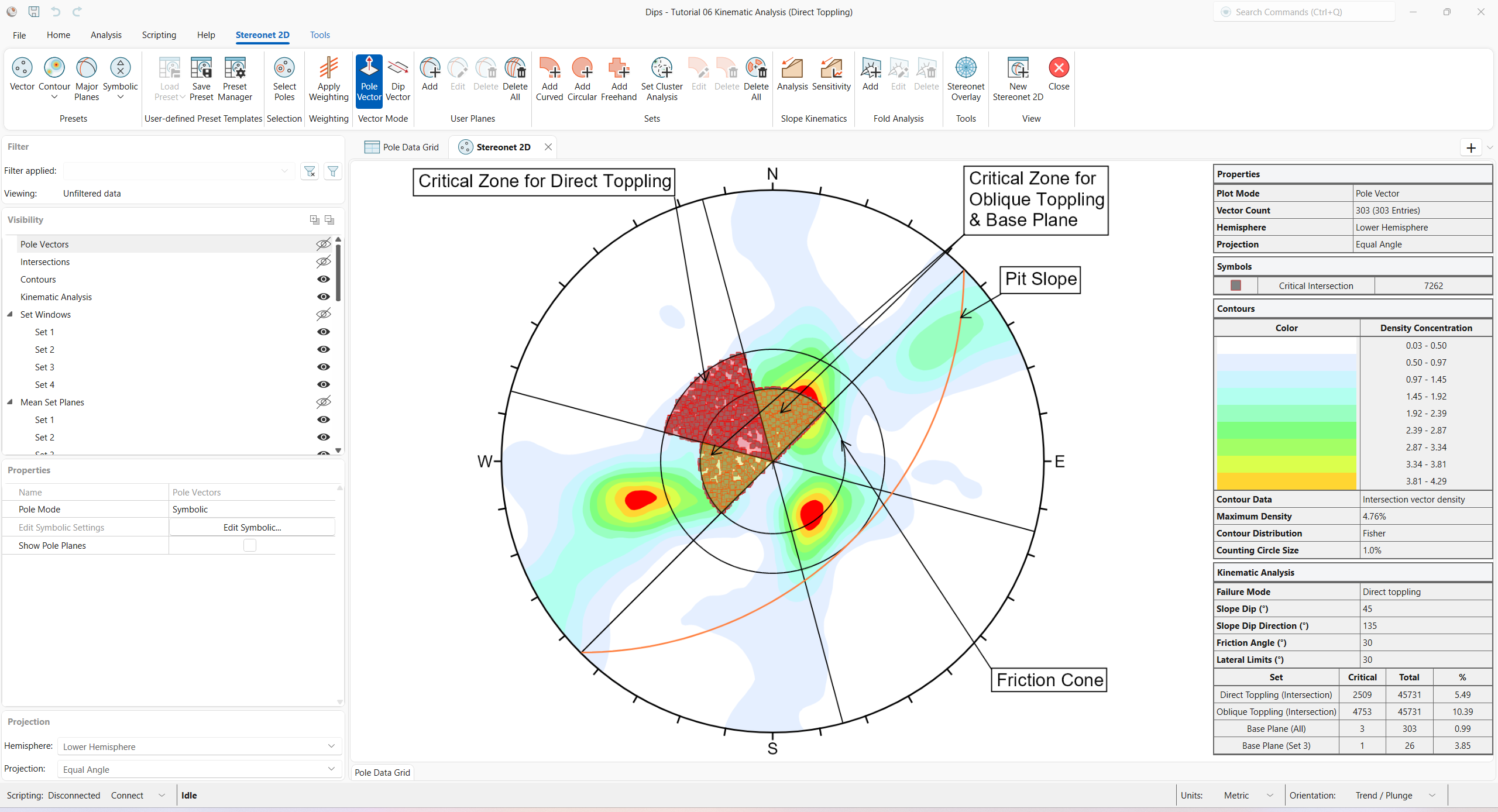
5.4.1 Friction Cone
For Direct Toppling, it is important to remember that the Friction Cone (30 degrees) is measured from the CENTER of the stereonet.
5.4.2 Lateral Limits
The same Lateral Limits (30 degrees) are used.
5.4.3 Critical Zone For Flexural Toppling
The Primary Critical Zone for Direct Toppling is the highlighted red (intersections and base plane poles).
The Secondary Critical Zone is the highlighted yellow region where we consider oblique toppling (intersections and base plane poles).
5.4.4 Kinematic Analysis Legend (Results)
A summary of the Direct Toppling results is displayed in the Legend.
The Legend provides results as a percentage of all intersections for Direct Toppling (2509/45731) and Oblique Toppling (4753/45731).
Planes can also act as release planes (and sliding planes) at the base. These are reported for all poles in the Pole Data Grid (3/303), and as a percentage of poles for individual sets (1/26 for Set 3).
6.0 Sensitivity Analysis
The Kinematic Sensitivity option in DIPS makes it easy to perform sensitivity analysis by varying the main input parameters (Slope Angle, Slope Dip Direction, Friction Angle, and/or Lateral Limits) and plotting the results for each Failure Mode.
To generate a Kinematic Sensitivity chart:
- Select Stereonet 2D > Slope Kinematics > Sensitivity
 from the ribbon. The Kinematic Sensitivity
dialog opens.
from the ribbon. The Kinematic Sensitivity
dialog opens. - Set the Failure Mode = Wedge Sliding.
- Select the Slope Dip checkbox.
- Set the Slope Dip range From = 45 degrees, To = 90 degrees, at Interval = 1 degrees.
- Set the Intersection Type = Pole.
- Set the Chart Type = Cartesian (X, Y).
- Set the Vertical Axis = Percent.
Kinematic Sensitivity dialog - Click OK to create a Kinematic Sensitivity chart.
From examining the Sensitivity Plots, we get an increase in the percentage of possible Kinematic Wedge Sliding failures as the Slope Dip becomes steeper.

To generate another Kinematic Sensitivity chart:
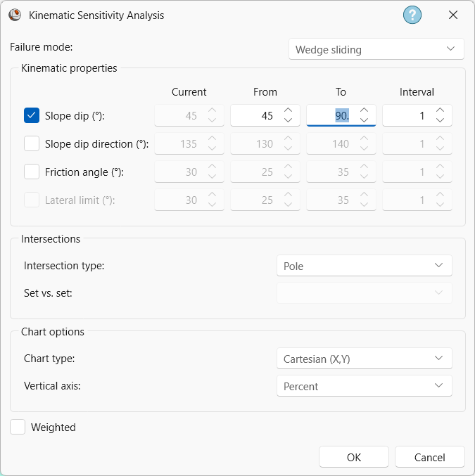
- Select Stereonet 2D > Slope Kinematics > Sensitivity from the ribbon. The Kinematic Sensitivity dialog opens.
- Set the Failure Mode = Wedge Sliding.
- Select the Slope Dip Direction checkbox.
- Set the Slope Dip Direction range From = 90 degrees, To = 180 degrees, at Interval = 1 degrees.
- Set the Intersection Type = Pole.
- Set the Chart Type = Cartesian (X, Y).
- Set the Vertical Axis = Percent.

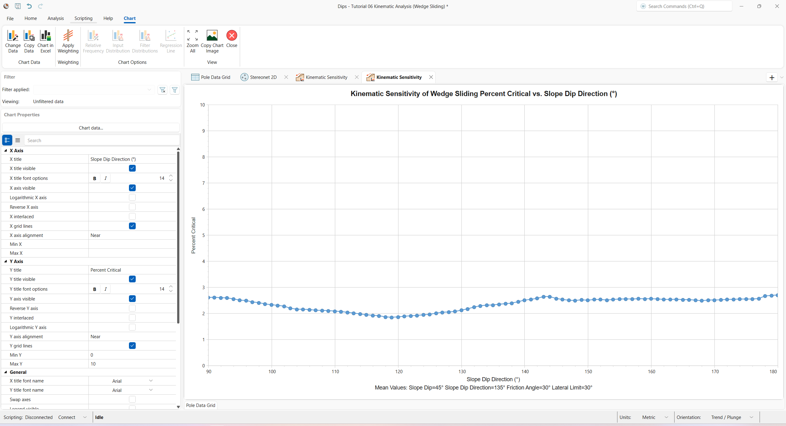
Kinematic Sensitivity dialog - Click OK to create a Kinematic Sensitivity chart.
The Slope Dip Direction has minimal effect on the percentage of possible Kinematic Wedge Sliding failures (less than 3%).
7.0 Terzaghi Weighting
It is important to note the effect of the Terzaghi Weighting on the Kinematic Analysis results.
If the Terzaghi Weighting is applied (Stereonet 2D > Weighting > Apply Weighting), the effect of bias correction on the Kinematic Analysis results will be accounted for, and the Kinematic Analysis results will be reported in terms of weighted counts of poles or intersections.
The weighting is applied to each pole based on the angle between the plane and the Traverse on which the data was collected, and all pole counts and “critical percent” values for all failure modes are reported using the weighted count values.
As an optional exercise, toggle the Apply Weighting ON and OFF to see the effect of applying bias correction on Mean Set Planes, Contours, and Critical %.
8.0 Summary
Kinematic Analysis of rock slope failure modes using stereonets is an extremely useful and easy-to-understand analysis tool which allows you to quickly evaluate potential failure modes. However, keep in mind the following.
- The analyses presented here are just a starting point for more detailed analysis and should always be accompanied by a more thorough field analysis in cases where a risk of failure is indicated.
- Real slopes may exhibit more than one failure mode. It is rare to see pure examples of these failure modes, particularly with the toppling analysis, which may exhibit complex behaviours involving sliding, toppling, rotating, etc.
- Even if a Kinematic Analysis indicates risk of failure, this does not necessarily mean that failure will occur, since factors other than kinematics and friction angle may work to increase stability (e.g. joint cohesion, joint persistence, etc). Conversely, other factors may decrease the stability (e.g. water pressure) of kinematically safe slopes.
- It is important to look beyond statistical results (e.g. mean set plane orientations) and consider major discrete structures such as shear zones, which may have a dominant effect on stability due to low friction angles and inherent persistence.
- More detailed analysis, including safety factor calculation, can be carried out with the Rocscience programs RocSlope2 and RocSlope3 (or UnWedge and RocTunnel3 for underground excavations).
9.0 References
- Goodman, R.E. 1980. Introduction to Rock Mechanics (Chapter 8), Toronto: John Wiley, pp 254-287.
- Hudson, J.A. and Harrison, J.P. 1997. Engineering Rock Mechanics – An Introduction to the Principles, Pergamon Press.
This concludes the tutorial. You are now ready for the next tutorial, Tutorial 07 – Curved Borehole Oriented Core.